MBOPT - Mass Balance Optimizer
MBOPT is a library for simulating and optimizing chemical process flowsheets modelled by mass balances only (i.e., there are no energy balance equations). The library is designed to be called from Lua, a simple and easy-to-learn scripting language. It can also be invoked from the command line by passing a Lua script as an argument. The library provides Lua functions to build, solve, and interact with the system of variables and equations that model a flowsheet. It uses Ipopt as the solver.
Objects
The library exposes objects to Lua. Each object is a member of a class. The classes of objects used in an MBOPT model are:
- Model: Contains objects of all of the other classes in this list and provides methods to build, manipulate, and solve a model.
- Flowsheet: Contains Streams, Blocks, Calcs, and other Flowsheets. A Model contains a single root Flowsheet that has zero or more trees of Flowsheets descending from it. A Flowsheet provides a namespace for the Streams, Blocks, Calcs, Variables, and Constraints that it contains. There can be a Stream named
feedor a Block namedheaderin more than one Flowsheet. - Stream: Contains a list of component names, like
h2,c2h4,naphtha, etc. Blocks use Streams to generate Variables that represent the total mass flow rates, component mass flow rates, and mass fractions of the Streams flowing into or out of the Block. The Variables associated with a Stream are contained in the Blocks that use that Stream as an inlet or an outlet. The Streams themselves contain only component names. - Block: Contains the Streams, Variables, Constraints, JacobianNZs, and HessianNZs (NZ = nonzero) that model a single unit operation. Available Blocks are:
- Mixer: Mixes two or more inlet Streams and produces a single outlet Stream.
- Splitter: Splits a single inlet Stream into two or more outlet Streams. The outlet Streams have the same composition as the inlet Stream.
- Separator: Separates each component in a single inlet stream into two or more outlet streams. A component may go into only one outlet stream, or specified fractions of the component may go into each outlet stream. A Separator models the mass balances in a distillation column, flash drum, or similar unit operation.
- YieldReactor: Converts the components in a single inlet stream into the components in a single outlet stream using specified fractional yields.
- MultiYieldReactor: Models a set of YieldReactors operating in parallel with two or more named feedstocks. Each YieldReactor in the set has one inlet stream and one outlet stream associated with each named feedstock.
- StoicReactor: Models a reactor with one inlet stream and one outlet stream in which the inlet stream components undergo a set of irreversible reactions with specified stoichiometry and fractional conversions.
- Calc: Used to create Variables, Constraints, JacobianNZs, and HessianNZs that relate Block and Calc Variables to each other. A simple example is a Calc to calculate the overall mass balance around a Flowsheet. A Calc does not have Streams associated with it. Calc blocks are implemented entirely in Lua.
- Quantity: An object with a value and a Unit. Objects like Variables, Prices, and Objectives are Quantities that have additional properties, e.g., Variables have names, lower bounds, and upper bounds. These derived objects are always contained in a Model, but standalone Quantity objects can be created and used for calculations.
- Variable: A Variable is a Quantity used to represent a variable in the system of equations contained in a Model. A Variable has a name, value, lower bound, upper bound, specification (fixed or free), and Unit associated with it. Variables are contained in a Model, but Blocks and Calcs hold pointers to their Variables.
- Constraint: Constraints represent the equality constraints (equations) contained in a Model. A Constraint has a name and a value, but no Unit. Constraints have the form $g(x_1, x_2, ..., x_n)=0$, where the $x_i$ are Variables and $g$ is an algebraic function of the $x_i$. MBOPT supports only simple bounds on Variables, not general inequality constraints.
- Objective: Objectives are Quantities that represent linear combinations of variables where each term in the linear combination is a Price multiplied by a Variable. The terms are objects called ObjTerms. Each ObjTerm has a scale factor associated with, which is normally either $+1$ or $-1$, but can be any number. This allows costs to be calculated without using negative Prices. Each Objective is made up of ObjTerms and other Objectives, forming a tree structure. The tree is contained in a Model, and the root Objective of the tree is used as the objective function by the solver.
- Price: A Quantity representing a material price. Prices are constants, not variables.
- Unit: A unit of measure, like "kg/hr" or "massfrac." Every Unit has a UnitKind, like massflow or massfrac (the name of a Unit can be the same as the name of its UnitKind). The string describing a Unit must be unique; there can't be two Units named "kg/hr" even if they have different UnitKinds. Quantities that have different Units with the same UnitKind can be converted to each other, and a Quantity can be expressed in any of the Units with the same UnitKind. Each UnitKind has a base Unit. The values of Variables are converted to base Units when used in arithmetic expressions to evaluate Constraints. The calculated value of the Constraint is a number with no Unit. Each UnitKind also has a default unit. When Variables of a specific UnitKind are created they are assigned the default unit for that UnitKind. Usually the base Unit and the default Unit are the same.
- UnitSet: Contains a set of Units. A Model has a single UnitSet and all Quantities in the Model like Variables and Objectives have Units drawn from the Model's UnitSet.
- Solver: Provides an interface to the Ipopt solver. A Solver object can set Ipopt options and solve a Model.
Getting Started
Working with Units and Quantities
Our goal is to build a mass balance model, solve it, and analyze the results. The model needs a UnitSet that defines the Units assigned to Variables, Prices, and Objectives. There are two ways to create a UnitSet: 1) create an empty UnitSet and then add UnitKinds and Units individually, and 2) describe the entire UnitSet in a single Lua table. Here we'll use option 1:
require "mboptlib" -- load the MBOPT library
us = UnitSet() -- create an empty UnitSet
us:add_kind("massflow", "kg/hr")     -- If "kg/hr" is not already in the UnitSet, it will be created
us:add_kind("massfrac", "massfrac")  --     and used as the base Unit for the new UnitKind.
print(us)
┌────────────┬────────────┬──────────────┬──────────────┬──────┬─────────┐
│    Unit    │    Kind    │     Ratio    │    Offset    │ Base │ Default │
├────────────┼────────────┼──────────────┼──────────────┼──────┼─────────┤
│kg/hr       │massflow    │             1│             0│   x  │    x    │
│massfrac    │massfrac    │             1│             0│   x  │    x    │
└────────────┴────────────┴──────────────┴──────────────┴──────┴─────────┘
2 Units shown
The first argument to add_kind is the name of the UnitKind. The second argument is the base Unit for that UnitKind. If the base Unit doesn't already exist it will be created (by definition, the base Unit has a ratio of 1 and offset of 0). If the default Unit isn't specified in the third argument it will be set to the base Unit. Any subsequently created Unit of the same UnitKind must be assigned a ratio and an offset. The offset defaults to 0. A Quantity has a value and a Unit. The value of a Quantity can be converted from its value in its native Unit to its value in the base Unit by multiplying by native Unit's ratio and adding the offset. In mass balance models the offset is always 0.
Here's how to add Units to a UnitSet:
us:add_unit("massflow", "lb/hr", 1.0 / 2.20462)   -- args are UnitKind name, Unit string, and unit ratio
us:add_unit("massflow", "t/hr", 1000.0, 0.0)      --    unit offset is the optional 4th arg, which defaults to 0.
us:add_unit("massfrac", "mass%", 1.0 / 100.0)
print(us)
┌────────────┬────────────┬──────────────┬──────────────┬──────┬─────────┐
│    Unit    │    Kind    │     Ratio    │    Offset    │ Base │ Default │
├────────────┼────────────┼──────────────┼──────────────┼──────┼─────────┤
│kg/hr       │massflow    │             1│             0│   x  │    x    │
│lb/hr       │massflow    │     0.4535929│             0│      │         │
│t/hr        │massflow    │          1000│             0│      │         │
│mass%       │massfrac    │          0.01│             0│      │         │
│massfrac    │massfrac    │             1│             0│   x  │    x    │
└────────────┴────────────┴──────────────┴──────────────┴──────┴─────────┘
5 Units shown
We can see from the table above that to convert a value in t/hr to kg/hr we multiply the value by 1000 and add 0, and to convert a value in mass% to massfrac we multiply by 0.01 and add 0. We can look up Units and UnitKinds in the UnitSet and get their properties:
u_lbhr = us.units["lb/hr"]
uk_massflow = us.kinds["massflow"]
print(u_lbhr)
print(uk_massflow)
print(u_lbhr.kind)
print(u_lbhr.ratio)
print(uk_massflow.base_unit)
lb/hr, kind=massflow
kind=massflow, base Unit=kg/hr, default Unit=kg/hr
kind=massflow, base Unit=kg/hr, default Unit=kg/hr
0.45359290943564
kg/hr, kind=massflow
Quantity objects combine a value and a Unit:
q1 = Quantity(1.0, us.units["kg/hr"])
print(type(q1))        -- can show the type of a Quantity
q2 = Q(1.0, u_lbhr)    -- can use Q instead of Quantity if desired
print("q1 = ", q1)
print("q2 = ", q2)
Quantity
q1 =               1_kg/hr
q2 =               1_lb/hr
A Quantity has .value and .unit properties:
print(q1.value)
print(q2.unit)
1.0
lb/hr, kind=massflow
You can assign to these properties:
q1.value = 2.0    -- q1's native Unit is kg/hr, so this makes q1 = 2 kg/hr
q1.unit = "lb/hr" -- Change q1's native Unit from kg/hr to lb/hr. This converts the existing value to lb/hr.
q2.v = 2.0        -- Can use v instead of value.
print("q1 = ", q1)
print("q2 = ", q2)
q1 =         4.40924_lb/hr
q2 =               2_lb/hr
Be careful not to assign a number to a Quantity, assuming it will assign the number to the value attribute of the Quantity. Instead, the variable will now be a number, no longer a Quantity. To illustrate:
quan = Quantity(1.0, us.units["kg/hr"])
print(type(quan))
quan = 5.0    -- wrong! this doesn't assign 5.0 to quan.value, it binds 5.0 (a number) to quan
print(type(quan))
Quantity
number
We can do arithmetic on Quantities:
res = q1 + q2    -- res is not a Quantity, it's a number
print(res)
print(type(res))
2.9071858188713
number
We see that the result is a number, not a Quantity. Furthermore, when a Quantity is used in an arithmetic expression its value is first converted to its base unit, and the base value of the Quantity is used in the expression. The result of the expression is a number without a Unit. It's the user's responsibility to maintain dimensional consistency and properly interpret the results of arithmetic expressions involving Quantities. This was a deliberate design choice; it greatly simplifies the implementation of units.
We can evaluate q1 - q2 directly and then confirm that the result is the same as subtracting the base value of q2 from the base value of q1::
print(q1 - q2)
print(q1.base_value - q2.bv)    -- can use bv instead of base_value
1.0928141811287
1.0928141811287
We can multiply and divide Quantities of different kinds, e.g., we can multiply a massflow by a massfrac to calculate a component mass flow rate. That operation makes sense. Multiplying a massflow by another massflow, on the other hand, rarely makes sense, but the MBOPT library does not prevent it.
Here's an example:
print("q1.value = ", q1.v, q1.unit.str)
print("q1.base_value = ", q1.bv, q1.base_unit.str)

q2 = Q(0.5, us.units["massfrac"])
print("q2.value = ", q2.v, q2.unit.str)
print("q2.base_value = ", q2.bv, q2.base_unit.str)

q3 = Q(q1 * q2, q1.base_unit)
print("q3 = q1 * q2 = ", q3)
print("q3 = ", q3:value_in(u_lbhr), u_lbhr.str)    -- value_in returns the value in the specified Unit

q4 = Q(q3)    -- can construct a new Quantity from an existing one
print("q4 = ", q4)
q1.value =  4.40924 lb/hr
q1.base_value =  2.0 kg/hr
q2.value =  0.5 massfrac
q2.base_value =  0.5 massfrac
q3 = q1 * q2 =               1_kg/hr
q3 =  0.45359290943564 lb/hr
q4 =               1_kg/hr
Building and Solving a Model
For our first Model we'll load a more extensive UnitSet from a file:
us = dofile("unitset.lua")
print(us)
┌────────────┬────────────┬──────────────┬──────────────┬──────┬─────────┐
│    Unit    │    Kind    │     Ratio    │    Offset    │ Base │ Default │
├────────────┼────────────┼──────────────┼──────────────┼──────┼─────────┤
│#           │count       │             1│             0│   x  │    x    │
│$/day       │flowval     │    0.04166667│             0│      │         │
│$/hr        │flowval     │             1│             0│   x  │    x    │
│%           │frac        │          0.01│             0│      │         │
│frac        │frac        │             1│             0│   x  │    x    │
│kg/hr       │massflow    │             1│             0│   x  │    x    │
│lb/hr       │massflow    │     0.4535929│             0│      │         │
│t/hr        │massflow    │          1000│             0│      │         │
│mass%       │massfrac    │          0.01│             0│      │         │
│massfrac    │massfrac    │             1│             0│   x  │    x    │
│$/kg        │massval     │             1│             0│   x  │    x    │
│$/lb        │massval     │       2.20462│             0│      │         │
│cts/lb      │massval     │     0.0220462│             0│      │         │
│kmol/hr     │moleflow    │             1│             0│   x  │    x    │
│kg/kmol     │molewt      │             1│             0│   x  │    x    │
└────────────┴────────────┴──────────────┴──────────────┴──────┴─────────┘
15 Units shown
We create an empty Model by specifying a name for the Model, a name for the root Flowsheet (usually named the "index" Flowsheet), and a UnitSet:
m = Model("demo", "index", us)    -- args are: Model name, root Flowsheet name, UnitSet
print(m)
Model: demo
  Number of equations          = 0
  Number of free variables     = 0
  Number of fixed variables    = 0
  Number of variables          = 0
  Number of Jacobian non-zeros = 0
  Number of Hessian non-zeros  = 0
Model is square
The index Flowsheet will be used to contain the Streams and Blocks that make up the model:
fs = m.index_fs
We'll create a Mixer block and the Streams that flow through it:
comps_in1 = {"c1", "c2"}       -- component names
comps_in2 = {"c1", "c2", "c3"}
comps_out = comps_in2    -- a Mixer outlet stream component list must equal the union of the inlet stream component lists

strm_in1, strm_in2, strm_out = fs:Streams(
    {"in1", comps_in1},
    {"in2", comps_in2},
    {"out", comps_out}
)

mix1 = fs:Mixer("mix1", {strm_in1, strm_in2}, {strm_out})    -- args are: block name, table of inlet streams, table of outlet streams

print(strm_in1)
print(strm_in2)
print(strm_out)
print(mix1)
print(fs)
Stream: in1
  flowsheet: index
  from: nil
  to: mix1
  comps: c1 c2

Stream: in2
  flowsheet: index
  from: nil
  to: mix1
  comps: c1 c2 c3

Stream: out
  flowsheet: index
  from: mix1
  to: nil
  comps: c1 c2 c3

Block: mix1
  type: Mixer
  flowsheet: index
  in:  in1 in2
  out: out


Flowsheet: index
  Blocks:
    mix1         (Mixer)              in: in1 in2   out: out
mix1:show_variables() -- show the variables in the mix1 block
┌─────┬────────────────────────────────┬───┬──────────────┬──────────────┬──────────────┬────────┐
│Index│              Name              │Fix│     Value    │     Lower    │     Upper    │  Unit  │
├─────┼────────────────────────────────┼───┼──────────────┼──────────────┼──────────────┼────────┤
│    0│mix1.in1.mass                   │   │             0│              │              │kg/hr   │
│    1│mix1.in1.mass_c1                │ = │             0│              │              │kg/hr   │
│    2│mix1.in1.mass_c2                │ = │             0│              │              │kg/hr   │
│    3│mix1.in1.massfrac_c1            │   │             0│              │              │massfrac│
│    4│mix1.in1.massfrac_c2            │   │             0│              │              │massfrac│
│    5│mix1.in2.mass                   │   │             0│              │              │kg/hr   │
│    6│mix1.in2.mass_c1                │ = │             0│              │              │kg/hr   │
│    7│mix1.in2.mass_c2                │ = │             0│              │              │kg/hr   │
│    8│mix1.in2.mass_c3                │ = │             0│              │              │kg/hr   │
│    9│mix1.in2.massfrac_c1            │   │             0│              │              │massfrac│
│   10│mix1.in2.massfrac_c2            │   │             0│              │              │massfrac│
│   11│mix1.in2.massfrac_c3            │   │             0│              │              │massfrac│
│   12│mix1.out.mass                   │   │             0│              │              │kg/hr   │
│   13│mix1.out.mass_c1                │   │             0│              │              │kg/hr   │
│   14│mix1.out.mass_c2                │   │             0│              │              │kg/hr   │
│   15│mix1.out.mass_c3                │   │             0│              │              │kg/hr   │
│   16│mix1.out.massfrac_c1            │   │             0│              │              │massfrac│
│   17│mix1.out.massfrac_c2            │   │             0│              │              │massfrac│
│   18│mix1.out.massfrac_c3            │   │             0│              │              │massfrac│
└─────┴────────────────────────────────┴───┴──────────────┴──────────────┴──────────────┴────────┘
19 Variables shown
All newly created Variables start with their values set to 0. A Variable's initial specification depends on the context. In all Blocks the component mass flow rates of the inlet streams are initially fixed variables (note the = sign in the Fix column). In a Mixer all the other variables are free. To calculate initial guesses of the values of the free variables we have to specify values for the fixed variables using the eval method of the Model object:
m:eval([[
    mix1.in1.mass_c1 = 1.0   -- set all the component mass flow rates to 1
    mix1.in1.mass_c2 = 1.0
    mix1.in2.mass_c1 = 1.0
    mix1.in2.mass_c2 = 1.0
    mix1.in2.mass_c3 = 1.0
]])

m:show_variables()    -- show the variables in the model, which so far contains only the mix1 block
┌─────┬────────────────────────────────┬───┬──────────────┬──────────────┬──────────────┬────────┐
│Index│              Name              │Fix│     Value    │     Lower    │     Upper    │  Unit  │
├─────┼────────────────────────────────┼───┼──────────────┼──────────────┼──────────────┼────────┤
│    0│mix1.in1.mass                   │   │             0│              │              │kg/hr   │
│    1│mix1.in1.mass_c1                │ = │             1│              │              │kg/hr   │
│    2│mix1.in1.mass_c2                │ = │             1│              │              │kg/hr   │
│    3│mix1.in1.massfrac_c1            │   │             0│              │              │massfrac│
│    4│mix1.in1.massfrac_c2            │   │             0│              │              │massfrac│
│    5│mix1.in2.mass                   │   │             0│              │              │kg/hr   │
│    6│mix1.in2.mass_c1                │ = │             1│              │              │kg/hr   │
│    7│mix1.in2.mass_c2                │ = │             1│              │              │kg/hr   │
│    8│mix1.in2.mass_c3                │ = │             1│              │              │kg/hr   │
│    9│mix1.in2.massfrac_c1            │   │             0│              │              │massfrac│
│   10│mix1.in2.massfrac_c2            │   │             0│              │              │massfrac│
│   11│mix1.in2.massfrac_c3            │   │             0│              │              │massfrac│
│   12│mix1.out.mass                   │   │             0│              │              │kg/hr   │
│   13│mix1.out.mass_c1                │   │             0│              │              │kg/hr   │
│   14│mix1.out.mass_c2                │   │             0│              │              │kg/hr   │
│   15│mix1.out.mass_c3                │   │             0│              │              │kg/hr   │
│   16│mix1.out.massfrac_c1            │   │             0│              │              │massfrac│
│   17│mix1.out.massfrac_c2            │   │             0│              │              │massfrac│
│   18│mix1.out.massfrac_c3            │   │             0│              │              │massfrac│
└─────┴────────────────────────────────┴───┴──────────────┴──────────────┴──────────────┴────────┘
19 Variables shown
Now we can initialize the model:
m:init()    -- calculates the values of the free variables
m:show_variables()
┌─────┬────────────────────────────────┬───┬──────────────┬──────────────┬──────────────┬────────┐
│Index│              Name              │Fix│     Value    │     Lower    │     Upper    │  Unit  │
├─────┼────────────────────────────────┼───┼──────────────┼──────────────┼──────────────┼────────┤
│    0│mix1.in1.mass                   │   │             2│              │              │kg/hr   │
│    1│mix1.in1.mass_c1                │ = │             1│              │              │kg/hr   │
│    2│mix1.in1.mass_c2                │ = │             1│              │              │kg/hr   │
│    3│mix1.in1.massfrac_c1            │   │           0.5│              │              │massfrac│
│    4│mix1.in1.massfrac_c2            │   │           0.5│              │              │massfrac│
│    5│mix1.in2.mass                   │   │             3│              │              │kg/hr   │
│    6│mix1.in2.mass_c1                │ = │             1│              │              │kg/hr   │
│    7│mix1.in2.mass_c2                │ = │             1│              │              │kg/hr   │
│    8│mix1.in2.mass_c3                │ = │             1│              │              │kg/hr   │
│    9│mix1.in2.massfrac_c1            │   │     0.3333333│              │              │massfrac│
│   10│mix1.in2.massfrac_c2            │   │     0.3333333│              │              │massfrac│
│   11│mix1.in2.massfrac_c3            │   │     0.3333333│              │              │massfrac│
│   12│mix1.out.mass                   │   │             5│              │              │kg/hr   │
│   13│mix1.out.mass_c1                │   │             2│              │              │kg/hr   │
│   14│mix1.out.mass_c2                │   │             2│              │              │kg/hr   │
│   15│mix1.out.mass_c3                │   │             1│              │              │kg/hr   │
│   16│mix1.out.massfrac_c1            │   │           0.4│              │              │massfrac│
│   17│mix1.out.massfrac_c2            │   │           0.4│              │              │massfrac│
│   18│mix1.out.massfrac_c3            │   │           0.2│              │              │massfrac│
└─────┴────────────────────────────────┴───┴──────────────┴──────────────┴──────────────┴────────┘
19 Variables shown
After initializing, if we evaluate the constraints their values should all be zero:
m:eval_constraints()
m:show_constraints()
┌─────┬────────────────────────────────┬──────────────┐
│Index│              Name              │     Value    │
├─────┼────────────────────────────────┼──────────────┤
│    0│mix1.c1_mass_balance            │             0│
│    1│mix1.c2_mass_balance            │             0│
│    2│mix1.c3_mass_balance            │             0│
│    3│mix1.in1_total_mass_def         │             0│
│    4│mix1.in2_total_mass_def         │             0│
│    5│mix1.out_total_mass_def         │             0│
│    6│mix1.in1.c1_massfrac_def        │             0│
│    7│mix1.in1.c2_massfrac_def        │             0│
│    8│mix1.in2.c1_massfrac_def        │ -5.551115e-17│
│    9│mix1.in2.c2_massfrac_def        │ -5.551115e-17│
│   10│mix1.in2.c3_massfrac_def        │ -5.551115e-17│
│   11│mix1.out.c1_massfrac_def        │  1.110223e-16│
│   12│mix1.out.c2_massfrac_def        │  1.110223e-16│
│   13│mix1.out.c3_massfrac_def        │  5.551115e-17│
└─────┴────────────────────────────────┴──────────────┘
14 Constraints shown
Changing the value of a Variable without reinitializing the block or the model should result in one or more constraints becoming nonzero:
m:get("mix1.in1.mass_c1").v = 2.0    -- use the get method to retrieve a Variable by name
mix1:eval_constraints()              -- can evaluate the constraints in a specific block
m:show_constraints()
┌─────┬────────────────────────────────┬──────────────┐
│Index│              Name              │     Value    │
├─────┼────────────────────────────────┼──────────────┤
│    0│mix1.c1_mass_balance            │             1│
│    1│mix1.c2_mass_balance            │             0│
│    2│mix1.c3_mass_balance            │             0│
│    3│mix1.in1_total_mass_def         │             1│
│    4│mix1.in2_total_mass_def         │             0│
│    5│mix1.out_total_mass_def         │             0│
│    6│mix1.in1.c1_massfrac_def        │            -1│
│    7│mix1.in1.c2_massfrac_def        │             0│
│    8│mix1.in2.c1_massfrac_def        │ -5.551115e-17│
│    9│mix1.in2.c2_massfrac_def        │ -5.551115e-17│
│   10│mix1.in2.c3_massfrac_def        │ -5.551115e-17│
│   11│mix1.out.c1_massfrac_def        │  1.110223e-16│
│   12│mix1.out.c2_massfrac_def        │  1.110223e-16│
│   13│mix1.out.c3_massfrac_def        │  5.551115e-17│
└─────┴────────────────────────────────┴──────────────┘
14 Constraints shown
To solve the model we first create a Solver object:
sv = Solver()
print(sv)
Ipopt
Set the tolerance and solve:
sv:set_option("tol", 1.0e-6)
sv:solve(m)
m:show_variables()
******************************************************************************
This program contains Ipopt, a library for large-scale nonlinear optimization.
 Ipopt is released as open source code under the Eclipse Public License (EPL).
         For more information visit https://github.com/coin-or/Ipopt
******************************************************************************

This is Ipopt version 3.14.19, running with linear solver MUMPS 5.6.2.

Number of nonzeros in equality constraint Jacobian...:       28
Number of nonzeros in inequality constraint Jacobian.:        0
Number of nonzeros in Lagrangian Hessian.............:        8

Total number of variables............................:       14
                     variables with only lower bounds:        0
                variables with lower and upper bounds:        0
                     variables with only upper bounds:        0
Total number of equality constraints.................:       14
Total number of inequality constraints...............:        0
        inequality constraints with only lower bounds:        0
   inequality constraints with lower and upper bounds:        0
        inequality constraints with only upper bounds:        0

iter    objective    inf_pr   inf_du lg(mu)  ||d||  lg(rg) alpha_du alpha_pr  ls
   0  1.0000000e+00 1.00e+00 0.00e+00  -1.0 0.00e+00    -  0.00e+00 0.00e+00   0
   1  1.0000000e+00 2.50e-01 0.00e+00  -1.7 1.00e+00    -  1.00e+00 1.00e+00h  1
   2  1.0000000e+00 1.11e-16 0.00e+00  -1.7 8.33e-02    -  1.00e+00 1.00e+00h  1

Number of Iterations....: 2

                                   (scaled)                 (unscaled)
Objective...............:   1.0000000000000000e+00    1.0000000000000000e+00
Dual infeasibility......:   0.0000000000000000e+00    0.0000000000000000e+00
Constraint violation....:   1.1102230246251565e-16    1.1102230246251565e-16
Variable bound violation:   0.0000000000000000e+00    0.0000000000000000e+00
Complementarity.........:   0.0000000000000000e+00    0.0000000000000000e+00
Overall NLP error.......:   1.1102230246251565e-16    1.1102230246251565e-16


Number of objective function evaluations             = 3
Number of objective gradient evaluations             = 3
Number of equality constraint evaluations            = 3
Number of inequality constraint evaluations          = 0
Number of equality constraint Jacobian evaluations   = 3
Number of inequality constraint Jacobian evaluations = 0
Number of Lagrangian Hessian evaluations             = 2
Total seconds in IPOPT                               = 0.004

EXIT: Optimal Solution Found.

┌─────┬────────────────────────────────┬───┬──────────────┬──────────────┬──────────────┬────────┐
│Index│              Name              │Fix│     Value    │     Lower    │     Upper    │  Unit  │
├─────┼────────────────────────────────┼───┼──────────────┼──────────────┼──────────────┼────────┤
│    0│mix1.in1.mass                   │   │             3│              │              │kg/hr   │
│    1│mix1.in1.mass_c1                │ = │             2│              │              │kg/hr   │
│    2│mix1.in1.mass_c2                │ = │             1│              │              │kg/hr   │
│    3│mix1.in1.massfrac_c1            │   │     0.6666667│              │              │massfrac│
│    4│mix1.in1.massfrac_c2            │   │     0.3333333│              │              │massfrac│
│    5│mix1.in2.mass                   │   │             3│              │              │kg/hr   │
│    6│mix1.in2.mass_c1                │ = │             1│              │              │kg/hr   │
│    7│mix1.in2.mass_c2                │ = │             1│              │              │kg/hr   │
│    8│mix1.in2.mass_c3                │ = │             1│              │              │kg/hr   │
│    9│mix1.in2.massfrac_c1            │   │     0.3333333│              │              │massfrac│
│   10│mix1.in2.massfrac_c2            │   │     0.3333333│              │              │massfrac│
│   11│mix1.in2.massfrac_c3            │   │     0.3333333│              │              │massfrac│
│   12│mix1.out.mass                   │   │             6│              │              │kg/hr   │
│   13│mix1.out.mass_c1                │   │             3│              │              │kg/hr   │
│   14│mix1.out.mass_c2                │   │             2│              │              │kg/hr   │
│   15│mix1.out.mass_c3                │   │             1│              │              │kg/hr   │
│   16│mix1.out.massfrac_c1            │   │           0.5│              │              │massfrac│
│   17│mix1.out.massfrac_c2            │   │     0.3333333│              │              │massfrac│
│   18│mix1.out.massfrac_c3            │   │     0.1666667│              │              │massfrac│
└─────┴────────────────────────────────┴───┴──────────────┴──────────────┴──────────────┴────────┘
19 Variables shown
Next we'll add a Splitter:
strm_s1, strm_s2 = fs:Streams(
    {"s1", {"c1", "c2", "c3"}},
    {"s2", {"c1", "c2", "c3"}}
)

spl1 = fs:Splitter("spl1", {strm_out}, {strm_s1, strm_s2})

print(strm_s1)
print(strm_s2)
print(spl1)
print(fs)

m:show_variables()
Stream: s1
  flowsheet: index
  from: spl1
  to: nil
  comps: c1 c2 c3

Stream: s2
  flowsheet: index
  from: spl1
  to: nil
  comps: c1 c2 c3

Block: spl1
  type: Splitter
  flowsheet: index
  in:  out
  out: s1 s2


Flowsheet: index
  Blocks:
    mix1         (Mixer)              in: in1 in2   out: out
    spl1         (Splitter)           in: out   out: s1 s2


┌─────┬────────────────────────────────┬───┬──────────────┬──────────────┬──────────────┬────────┐
│Index│              Name              │Fix│     Value    │     Lower    │     Upper    │  Unit  │
├─────┼────────────────────────────────┼───┼──────────────┼──────────────┼──────────────┼────────┤
│    0│mix1.in1.mass                   │   │             3│              │              │kg/hr   │
│    1│mix1.in1.mass_c1                │ = │             2│              │              │kg/hr   │
│    2│mix1.in1.mass_c2                │ = │             1│              │              │kg/hr   │
│    3│mix1.in1.massfrac_c1            │   │     0.6666667│              │              │massfrac│
│    4│mix1.in1.massfrac_c2            │   │     0.3333333│              │              │massfrac│
│    5│mix1.in2.mass                   │   │             3│              │              │kg/hr   │
│    6│mix1.in2.mass_c1                │ = │             1│              │              │kg/hr   │
│    7│mix1.in2.mass_c2                │ = │             1│              │              │kg/hr   │
│    8│mix1.in2.mass_c3                │ = │             1│              │              │kg/hr   │
│    9│mix1.in2.massfrac_c1            │   │     0.3333333│              │              │massfrac│
│   10│mix1.in2.massfrac_c2            │   │     0.3333333│              │              │massfrac│
│   11│mix1.in2.massfrac_c3            │   │     0.3333333│              │              │massfrac│
│   12│mix1.out.mass                   │   │             6│              │              │kg/hr   │
│   13│mix1.out.mass_c1                │   │             3│              │              │kg/hr   │
│   14│mix1.out.mass_c2                │   │             2│              │              │kg/hr   │
│   15│mix1.out.mass_c3                │   │             1│              │              │kg/hr   │
│   16│mix1.out.massfrac_c1            │   │           0.5│              │              │massfrac│
│   17│mix1.out.massfrac_c2            │   │     0.3333333│              │              │massfrac│
│   18│mix1.out.massfrac_c3            │   │     0.1666667│              │              │massfrac│
│   19│spl1.out.mass                   │   │             0│              │              │kg/hr   │
│   20│spl1.out.mass_c1                │ = │             0│              │              │kg/hr   │
│   21│spl1.out.mass_c2                │ = │             0│              │              │kg/hr   │
│   22│spl1.out.mass_c3                │ = │             0│              │              │kg/hr   │
│   23│spl1.out.massfrac_c1            │   │             0│              │              │massfrac│
│   24│spl1.out.massfrac_c2            │   │             0│              │              │massfrac│
│   25│spl1.out.massfrac_c3            │   │             0│              │              │massfrac│
│   26│spl1.s1.mass                    │   │             0│              │              │kg/hr   │
│   27│spl1.s1.mass_c1                 │   │             0│              │              │kg/hr   │
│   28│spl1.s1.mass_c2                 │   │             0│              │              │kg/hr   │
│   29│spl1.s1.mass_c3                 │   │             0│              │              │kg/hr   │
│   30│spl1.s1.massfrac_c1             │   │             0│              │              │massfrac│
│   31│spl1.s1.massfrac_c2             │   │             0│              │              │massfrac│
│   32│spl1.s1.massfrac_c3             │   │             0│              │              │massfrac│
│   33│spl1.s2.mass                    │   │             0│              │              │kg/hr   │
│   34│spl1.s2.mass_c1                 │   │             0│              │              │kg/hr   │
│   35│spl1.s2.mass_c2                 │   │             0│              │              │kg/hr   │
│   36│spl1.s2.mass_c3                 │   │             0│              │              │kg/hr   │
│   37│spl1.s2.massfrac_c1             │   │             0│              │              │massfrac│
│   38│spl1.s2.massfrac_c2             │   │             0│              │              │massfrac│
│   39│spl1.s2.massfrac_c3             │   │             0│              │              │massfrac│
│   40│spl1.s1.splitfrac               │ = │             0│              │              │frac    │
│   41│spl1.s2.splitfrac               │   │             0│              │              │frac    │
└─────┴────────────────────────────────┴───┴──────────────┴──────────────┴──────────────┴────────┘
42 Variables shown
We see that the spl1 inlet stream component mass flow rates are fixed variables. As we said earlier, newly created blocks start out with the inlet component mass flow rate variables fixed. The component mass flow rates of stream out in block mix1 are not connected to the component mass flow rate of stream out in block spl1. The blocks are uncoupled from each other. Usually we want to connect them, and that has to be done explicitly using the connect method. That method creates one or more Connections. Each Connection points to a constraint that sets two variables equal to each other. To make a Connection between two variables, one must be free and the other fixed, or both may be fixed, but attempting to connect two free variables will fail.
cnx1, cnx2, cnx3 = spl1:connect()    -- returns a list of Connections
print(cnx1)                   -- print them
print(cnx2)
print(cnx3)

m:show_connections()          -- show a table of the Connections made for stream out
spl1.out.mass_c1 = mix1.out.mass_c1
spl1.out.mass_c2 = mix1.out.mass_c2
spl1.out.mass_c3 = mix1.out.mass_c3

┌─────┬─────┬─────┬────────────────────────────────┬────────────────────────────────┬──────────────┐
│Index│ Var1│ Var2│            Variable 1          │            Variable 2          │    Value     │
├─────┼─────┼─────┼────────────────────────────────┼────────────────────────────────┼──────────────┤
│   33│   20│   13│spl1.out.mass_c1                │mix1.out.mass_c1                │             0│
│   34│   21│   14│spl1.out.mass_c2                │mix1.out.mass_c2                │             0│
│   35│   22│   15│spl1.out.mass_c3                │mix1.out.mass_c3                │             0│
└─────┴─────┴─────┴────────────────────────────────┴────────────────────────────────┴──────────────┘
3 connections shown
Now look at the variables in spl1:
spl1:show_variables()
┌─────┬────────────────────────────────┬───┬──────────────┬──────────────┬──────────────┬────────┐
│Index│              Name              │Fix│     Value    │     Lower    │     Upper    │  Unit  │
├─────┼────────────────────────────────┼───┼──────────────┼──────────────┼──────────────┼────────┤
│   19│spl1.out.mass                   │   │             0│              │              │kg/hr   │
│   20│spl1.out.mass_c1                │   │             3│              │              │kg/hr   │
│   21│spl1.out.mass_c2                │   │             2│              │              │kg/hr   │
│   22│spl1.out.mass_c3                │   │             1│              │              │kg/hr   │
│   23│spl1.out.massfrac_c1            │   │             0│              │              │massfrac│
│   24│spl1.out.massfrac_c2            │   │             0│              │              │massfrac│
│   25│spl1.out.massfrac_c3            │   │             0│              │              │massfrac│
│   26│spl1.s1.mass                    │   │             0│              │              │kg/hr   │
│   27│spl1.s1.mass_c1                 │   │             0│              │              │kg/hr   │
│   28│spl1.s1.mass_c2                 │   │             0│              │              │kg/hr   │
│   29│spl1.s1.mass_c3                 │   │             0│              │              │kg/hr   │
│   30│spl1.s1.massfrac_c1             │   │             0│              │              │massfrac│
│   31│spl1.s1.massfrac_c2             │   │             0│              │              │massfrac│
│   32│spl1.s1.massfrac_c3             │   │             0│              │              │massfrac│
│   33│spl1.s2.mass                    │   │             0│              │              │kg/hr   │
│   34│spl1.s2.mass_c1                 │   │             0│              │              │kg/hr   │
│   35│spl1.s2.mass_c2                 │   │             0│              │              │kg/hr   │
│   36│spl1.s2.mass_c3                 │   │             0│              │              │kg/hr   │
│   37│spl1.s2.massfrac_c1             │   │             0│              │              │massfrac│
│   38│spl1.s2.massfrac_c2             │   │             0│              │              │massfrac│
│   39│spl1.s2.massfrac_c3             │   │             0│              │              │massfrac│
│   40│spl1.s1.splitfrac               │ = │             0│              │              │frac    │
│   41│spl1.s2.splitfrac               │   │             0│              │              │frac    │
└─────┴────────────────────────────────┴───┴──────────────┴──────────────┴──────────────┴────────┘
23 Variables shown
One of the two split fractions is the only fixed variable (the split fractions are constrained to sum to 1, so the other split fraction is free). After we set the value of spl1.s1.splitfrac we can initialize spl:
split_frac = spl1:get("spl1.s1.splitfrac")    -- Blocks also provide a get method
split_frac.v = 0.5                            -- set its value by assigning to the .v (or .value) property
spl1:init()
spl1:show_variables()
┌─────┬────────────────────────────────┬───┬──────────────┬──────────────┬──────────────┬────────┐
│Index│              Name              │Fix│     Value    │     Lower    │     Upper    │  Unit  │
├─────┼────────────────────────────────┼───┼──────────────┼──────────────┼──────────────┼────────┤
│   19│spl1.out.mass                   │   │             6│              │              │kg/hr   │
│   20│spl1.out.mass_c1                │   │             3│              │              │kg/hr   │
│   21│spl1.out.mass_c2                │   │             2│              │              │kg/hr   │
│   22│spl1.out.mass_c3                │   │             1│              │              │kg/hr   │
│   23│spl1.out.massfrac_c1            │   │           0.5│              │              │massfrac│
│   24│spl1.out.massfrac_c2            │   │     0.3333333│              │              │massfrac│
│   25│spl1.out.massfrac_c3            │   │     0.1666667│              │              │massfrac│
│   26│spl1.s1.mass                    │   │             3│              │              │kg/hr   │
│   27│spl1.s1.mass_c1                 │   │           1.5│              │              │kg/hr   │
│   28│spl1.s1.mass_c2                 │   │             1│              │              │kg/hr   │
│   29│spl1.s1.mass_c3                 │   │           0.5│              │              │kg/hr   │
│   30│spl1.s1.massfrac_c1             │   │           0.5│              │              │massfrac│
│   31│spl1.s1.massfrac_c2             │   │     0.3333333│              │              │massfrac│
│   32│spl1.s1.massfrac_c3             │   │     0.1666667│              │              │massfrac│
│   33│spl1.s2.mass                    │   │             3│              │              │kg/hr   │
│   34│spl1.s2.mass_c1                 │   │           1.5│              │              │kg/hr   │
│   35│spl1.s2.mass_c2                 │   │             1│              │              │kg/hr   │
│   36│spl1.s2.mass_c3                 │   │           0.5│              │              │kg/hr   │
│   37│spl1.s2.massfrac_c1             │   │           0.5│              │              │massfrac│
│   38│spl1.s2.massfrac_c2             │   │     0.3333333│              │              │massfrac│
│   39│spl1.s2.massfrac_c3             │   │     0.1666667│              │              │massfrac│
│   40│spl1.s1.splitfrac               │ = │           0.5│              │              │frac    │
│   41│spl1.s2.splitfrac               │   │           0.5│              │              │frac    │
└─────┴────────────────────────────────┴───┴──────────────┴──────────────┴──────────────┴────────┘
23 Variables shown
If we don't change any variable values the model should solve on the first iteration:
sv:solve(m)
This is Ipopt version 3.14.19, running with linear solver MUMPS 5.6.2.

Number of nonzeros in equality constraint Jacobian...:       83
Number of nonzeros in inequality constraint Jacobian.:        0
Number of nonzeros in Lagrangian Hessian.............:       18

Total number of variables............................:       36
                     variables with only lower bounds:        0
                variables with lower and upper bounds:        0
                     variables with only upper bounds:        0
Total number of equality constraints.................:       36
Total number of inequality constraints...............:        0
        inequality constraints with only lower bounds:        0
   inequality constraints with lower and upper bounds:        0
        inequality constraints with only upper bounds:        0

iter    objective    inf_pr   inf_du lg(mu)  ||d||  lg(rg) alpha_du alpha_pr  ls
   0  1.0000000e+00 1.11e-16 0.00e+00  -1.0 0.00e+00    -  0.00e+00 0.00e+00   0

Number of Iterations....: 0

                                   (scaled)                 (unscaled)
Objective...............:   1.0000000000000000e+00    1.0000000000000000e+00
Dual infeasibility......:   0.0000000000000000e+00    0.0000000000000000e+00
Constraint violation....:   1.1102230246251565e-16    1.1102230246251565e-16
Variable bound violation:   0.0000000000000000e+00    0.0000000000000000e+00
Complementarity.........:   0.0000000000000000e+00    0.0000000000000000e+00
Overall NLP error.......:   1.1102230246251565e-16    1.1102230246251565e-16


Number of objective function evaluations             = 1
Number of objective gradient evaluations             = 1
Number of equality constraint evaluations            = 1
Number of inequality constraint evaluations          = 0
Number of equality constraint Jacobian evaluations   = 1
Number of inequality constraint Jacobian evaluations = 0
Number of Lagrangian Hessian evaluations             = 0
Total seconds in IPOPT                               = 0.000

EXIT: Optimal Solution Found.
0
Admittedly we can't do anything very interesting with a two-block model, but we can use it to show how to define an objective function and solve an optimization problem. We'll first define some Prices:
prices = m:Prices(
    {"price.s1", 2.0, "$/kg"},    -- name, value, Unit
    {"price.s2", 1.0, "$/kg"},
    {"price.in", 0.5, "$/kg"}
)
m:show_prices()
┌────────────────────────────────┬──────────────┬────────┐
│              Name              │     Value    │  Unit  │
├────────────────────────────────┼──────────────┼────────┤
│price.in                        │           0.5│$/kg    │
│price.s2                        │             1│$/kg    │
│price.s1                        │             2│$/kg    │
└────────────────────────────────┴──────────────┴────────┘
3 prices shown
The objective function profit will be profit = sales - costs, where sales and costs are also objective functions:
sales = m:add_objective("sales", "$/hr",
    {"s1_val", "spl1.s1.mass", "price.s1", "$/hr"},   -- an ObjTerm is a table: {term name, Variable, Price, Unit}
    {"s2_val", "spl1.s2.mass", "price.s2", "$/hr"}    --    the value of the term is Variable * Price
)

costs = m:add_objective("costs", "$/hr", -1.0,    -- note the -1.0 scale factor. If omitted, the scale factor = +1.0
    {"in1_val", "mix1.in1.mass", "price.in", "$/hr"},
    {"in2_val", "mix1.in2.mass", "price.in", "$/hr"}
)

profit = m:add_objective("profit", "$/hr",
    sales,    -- any term in the Objective can also be a previously defined Objective
    costs)

m.obj = profit        -- set the model's root objective function

m:eval_objective()
m:show_objective()

profit_before_opt = Q(profit)    -- save the value of profit
print("Profit before optimizing = ", profit_before_opt)
Objective: profit

┌────────────────────────┬────────────────────────────────┬────────────────────────┬──────────────┬────────┐
│          Term          │            Variable            │          Price         │    Value     │  Unit  │
├────────────────────────┼────────────────────────────────┼────────────────────────┼──────────────┼────────┤
│in2_val                 │mix1.in2.mass                   │price.in                │           1.5│$/hr    │
│in1_val                 │mix1.in1.mass                   │price.in                │           1.5│$/hr    │
│                   costs│                                │                        │            -3│$/hr    │
│s2_val                  │spl1.s2.mass                    │price.s2                │             3│$/hr    │
│s1_val                  │spl1.s1.mass                    │price.s1                │             6│$/hr    │
│                   sales│                                │                        │             9│$/hr    │
│                  profit│                                │                        │             6│$/hr    │
└────────────────────────┴────────────────────────────────┴────────────────────────┴──────────────┴────────┘

Profit before optimizing =               6_$/hr
We have to specify at least one degree of freedom and put some bounds on variables so that the optimization problem is not unbounded. If we want a fixed variable to be a degree of freedom we have to change its specification to free:
m:eval([[
    free mix1.in1.mass_c1     -- fix all but one massfrac, free the component mass flows
    free mix1.in1.mass_c2
    fix  mix1.in1.massfrac_c1

    free mix1.in2.mass_c1
    free mix1.in2.mass_c2
    free mix1.in2.mass_c3
    fix  mix1.in2.massfrac_c1
    fix  mix1.in2.massfrac_c2

    free spl1.s1.splitfrac    -- make the s1 splitfrac a degree of freedom

    mix1.in1.mass < 10_kg/hr  -- put bounds on the degrees of freedom
    mix1.in2.mass < 5_kg/hr
    spl1.s1.splitfrac < 0.9
]])

print(m)
m:show_variables()
Model: demo    Objective: profit
  Number of equations          = 36
  Number of free variables     = 39
  Number of fixed variables    = 3
  Number of variables          = 42
  Number of Jacobian non-zeros = 100
  Number of Hessian non-zeros  = 19
Model has 3 degrees of freedom


┌─────┬────────────────────────────────┬───┬──────────────┬──────────────┬──────────────┬────────┐
│Index│              Name              │Fix│     Value    │     Lower    │     Upper    │  Unit  │
├─────┼────────────────────────────────┼───┼──────────────┼──────────────┼──────────────┼────────┤
│    0│mix1.in1.mass                   │   │             3│              │            10│kg/hr   │
│    1│mix1.in1.mass_c1                │   │             2│              │              │kg/hr   │
│    2│mix1.in1.mass_c2                │   │             1│              │              │kg/hr   │
│    3│mix1.in1.massfrac_c1            │ = │     0.6666667│              │              │massfrac│
│    4│mix1.in1.massfrac_c2            │   │     0.3333333│              │              │massfrac│
│    5│mix1.in2.mass                   │   │             3│              │             5│kg/hr   │
│    6│mix1.in2.mass_c1                │   │             1│              │              │kg/hr   │
│    7│mix1.in2.mass_c2                │   │             1│              │              │kg/hr   │
│    8│mix1.in2.mass_c3                │   │             1│              │              │kg/hr   │
│    9│mix1.in2.massfrac_c1            │ = │     0.3333333│              │              │massfrac│
│   10│mix1.in2.massfrac_c2            │ = │     0.3333333│              │              │massfrac│
│   11│mix1.in2.massfrac_c3            │   │     0.3333333│              │              │massfrac│
│   12│mix1.out.mass                   │   │             6│              │              │kg/hr   │
│   13│mix1.out.mass_c1                │   │             3│              │              │kg/hr   │
│   14│mix1.out.mass_c2                │   │             2│              │              │kg/hr   │
│   15│mix1.out.mass_c3                │   │             1│              │              │kg/hr   │
│   16│mix1.out.massfrac_c1            │   │           0.5│              │              │massfrac│
│   17│mix1.out.massfrac_c2            │   │     0.3333333│              │              │massfrac│
│   18│mix1.out.massfrac_c3            │   │     0.1666667│              │              │massfrac│
│   19│spl1.out.mass                   │   │             6│              │              │kg/hr   │
│   20│spl1.out.mass_c1                │   │             3│              │              │kg/hr   │
│   21│spl1.out.mass_c2                │   │             2│              │              │kg/hr   │
│   22│spl1.out.mass_c3                │   │             1│              │              │kg/hr   │
│   23│spl1.out.massfrac_c1            │   │           0.5│              │              │massfrac│
│   24│spl1.out.massfrac_c2            │   │     0.3333333│              │              │massfrac│
│   25│spl1.out.massfrac_c3            │   │     0.1666667│              │              │massfrac│
│   26│spl1.s1.mass                    │   │             3│              │              │kg/hr   │
│   27│spl1.s1.mass_c1                 │   │           1.5│              │              │kg/hr   │
│   28│spl1.s1.mass_c2                 │   │             1│              │              │kg/hr   │
│   29│spl1.s1.mass_c3                 │   │           0.5│              │              │kg/hr   │
│   30│spl1.s1.massfrac_c1             │   │           0.5│              │              │massfrac│
│   31│spl1.s1.massfrac_c2             │   │     0.3333333│              │              │massfrac│
│   32│spl1.s1.massfrac_c3             │   │     0.1666667│              │              │massfrac│
│   33│spl1.s2.mass                    │   │             3│              │              │kg/hr   │
│   34│spl1.s2.mass_c1                 │   │           1.5│              │              │kg/hr   │
│   35│spl1.s2.mass_c2                 │   │             1│              │              │kg/hr   │
│   36│spl1.s2.mass_c3                 │   │           0.5│              │              │kg/hr   │
│   37│spl1.s2.massfrac_c1             │   │           0.5│              │              │massfrac│
│   38│spl1.s2.massfrac_c2             │   │     0.3333333│              │              │massfrac│
│   39│spl1.s2.massfrac_c3             │   │     0.1666667│              │              │massfrac│
│   40│spl1.s1.splitfrac               │   │           0.5│              │           0.9│frac    │
│   41│spl1.s2.splitfrac               │   │           0.5│              │              │frac    │
└─────┴────────────────────────────────┴───┴──────────────┴──────────────┴──────────────┴────────┘
42 Variables shown
By default the solver minimizes the objective function. To maximize it we set the solver option "obj_scaling_factor" to -1. We set another option that tells the solver the objective function is linear, so its gradient only has to be evaluated once:
sv:set_option("obj_scaling_factor", -1.0)
sv:set_option("grad_f_constant", "yes")

sv:solve(m)
m:show_variables()

profit_after_opt = Q(m.obj)
print("Profit after optimizing = ", profit_after_opt)
profit_delta = Q(profit_after_opt - profit_before_opt, m.obj.unit)
print("Profit delta =", profit_delta)
This is Ipopt version 3.14.19, running with linear solver MUMPS 5.6.2.

Number of nonzeros in equality constraint Jacobian...:       97
Number of nonzeros in inequality constraint Jacobian.:        0
Number of nonzeros in Lagrangian Hessian.............:       16

Total number of variables............................:       39
                     variables with only lower bounds:        0
                variables with lower and upper bounds:        0
                     variables with only upper bounds:        3
Total number of equality constraints.................:       36
Total number of inequality constraints...............:        0
        inequality constraints with only lower bounds:        0
   inequality constraints with lower and upper bounds:        0
        inequality constraints with only upper bounds:        0

iter    objective    inf_pr   inf_du lg(mu)  ||d||  lg(rg) alpha_du alpha_pr  ls
   0  6.0000000e+00 1.11e-16 2.94e-01  -1.0 0.00e+00    -  0.00e+00 0.00e+00   0
   1  1.0052381e+01 6.64e-01 6.23e+00  -1.0 2.60e+01    -  1.00e+00 1.24e-01f  1
   2  1.9845253e+01 4.11e-01 2.34e+00  -1.0 6.58e+00    -  1.00e+00 1.00e+00f  1
   3  2.0736631e+01 1.90e-02 4.99e-03  -1.0 6.00e-01    -  1.00e+00 1.00e+00h  1
   4  2.0992108e+01 5.31e-04 4.72e-05  -2.5 1.86e-01    -  1.00e+00 1.00e+00h  1
   5  2.0999550e+01 4.84e-07 1.08e-08  -3.8 5.73e-03    -  1.00e+00 1.00e+00h  1
   6  2.0999995e+01 2.09e-09 1.84e-11  -5.7 3.39e-04    -  1.00e+00 1.00e+00h  1
   7  2.1000000e+01 2.93e-13 9.09e-13  -7.0 4.01e-06    -  1.00e+00 1.00e+00h  1

Number of Iterations....: 7

                                   (scaled)                 (unscaled)
Objective...............:  -2.1000000087273023e+01    2.1000000087273023e+01
Dual infeasibility......:   9.0949470177292824e-13    9.0949470177292824e-13
Constraint violation....:   2.9293393014002877e-13    2.9293393014002877e-13
Variable bound violation:   3.5065038872517107e-08    3.5065038872517107e-08
Complementarity.........:   9.0908944983494818e-08    9.0908944983494818e-08
Overall NLP error.......:   9.0908944983494818e-08    9.0908944983494818e-08


Number of objective function evaluations             = 8
Number of objective gradient evaluations             = 1
Number of equality constraint evaluations            = 8
Number of inequality constraint evaluations          = 0
Number of equality constraint Jacobian evaluations   = 8
Number of inequality constraint Jacobian evaluations = 0
Number of Lagrangian Hessian evaluations             = 7
Total seconds in IPOPT                               = 0.005

EXIT: Optimal Solution Found.

┌─────┬────────────────────────────────┬───┬──────────────┬──────────────┬──────────────┬────────┐
│Index│              Name              │Fix│     Value    │     Lower    │     Upper    │  Unit  │
├─────┼────────────────────────────────┼───┼──────────────┼──────────────┼──────────────┼────────┤
│    0│mix1.in1.mass                   │   │            10│              │            10│kg/hr   │
│    1│mix1.in1.mass_c1                │   │      6.666667│              │              │kg/hr   │
│    2│mix1.in1.mass_c2                │   │      3.333333│              │              │kg/hr   │
│    3│mix1.in1.massfrac_c1            │ = │     0.6666667│              │              │massfrac│
│    4│mix1.in1.massfrac_c2            │   │     0.3333333│              │              │massfrac│
│    5│mix1.in2.mass                   │   │             5│              │             5│kg/hr   │
│    6│mix1.in2.mass_c1                │   │      1.666667│              │              │kg/hr   │
│    7│mix1.in2.mass_c2                │   │      1.666667│              │              │kg/hr   │
│    8│mix1.in2.mass_c3                │   │      1.666667│              │              │kg/hr   │
│    9│mix1.in2.massfrac_c1            │ = │     0.3333333│              │              │massfrac│
│   10│mix1.in2.massfrac_c2            │ = │     0.3333333│              │              │massfrac│
│   11│mix1.in2.massfrac_c3            │   │     0.3333333│              │              │massfrac│
│   12│mix1.out.mass                   │   │            15│              │              │kg/hr   │
│   13│mix1.out.mass_c1                │   │      8.333333│              │              │kg/hr   │
│   14│mix1.out.mass_c2                │   │             5│              │              │kg/hr   │
│   15│mix1.out.mass_c3                │   │      1.666667│              │              │kg/hr   │
│   16│mix1.out.massfrac_c1            │   │     0.5555556│              │              │massfrac│
│   17│mix1.out.massfrac_c2            │   │     0.3333333│              │              │massfrac│
│   18│mix1.out.massfrac_c3            │   │     0.1111111│              │              │massfrac│
│   19│spl1.out.mass                   │   │            15│              │              │kg/hr   │
│   20│spl1.out.mass_c1                │   │      8.333333│              │              │kg/hr   │
│   21│spl1.out.mass_c2                │   │             5│              │              │kg/hr   │
│   22│spl1.out.mass_c3                │   │      1.666667│              │              │kg/hr   │
│   23│spl1.out.massfrac_c1            │   │     0.5555556│              │              │massfrac│
│   24│spl1.out.massfrac_c2            │   │     0.3333333│              │              │massfrac│
│   25│spl1.out.massfrac_c3            │   │     0.1111111│              │              │massfrac│
│   26│spl1.s1.mass                    │   │          13.5│              │              │kg/hr   │
│   27│spl1.s1.mass_c1                 │   │           7.5│              │              │kg/hr   │
│   28│spl1.s1.mass_c2                 │   │           4.5│              │              │kg/hr   │
│   29│spl1.s1.mass_c3                 │   │           1.5│              │              │kg/hr   │
│   30│spl1.s1.massfrac_c1             │   │     0.5555556│              │              │massfrac│
│   31│spl1.s1.massfrac_c2             │   │     0.3333333│              │              │massfrac│
│   32│spl1.s1.massfrac_c3             │   │     0.1111111│              │              │massfrac│
│   33│spl1.s2.mass                    │   │           1.5│              │              │kg/hr   │
│   34│spl1.s2.mass_c1                 │   │     0.8333333│              │              │kg/hr   │
│   35│spl1.s2.mass_c2                 │   │           0.5│              │              │kg/hr   │
│   36│spl1.s2.mass_c3                 │   │     0.1666667│              │              │kg/hr   │
│   37│spl1.s2.massfrac_c1             │   │     0.5555556│              │              │massfrac│
│   38│spl1.s2.massfrac_c2             │   │     0.3333333│              │              │massfrac│
│   39│spl1.s2.massfrac_c3             │   │     0.1111111│              │              │massfrac│
│   40│spl1.s1.splitfrac               │   │           0.9│              │           0.9│frac    │
│   41│spl1.s2.splitfrac               │   │           0.1│              │              │frac    │
└─────┴────────────────────────────────┴───┴──────────────┴──────────────┴──────────────┴────────┘
42 Variables shown

Profit after optimizing =              21_$/hr
Profit delta =             15_$/hr
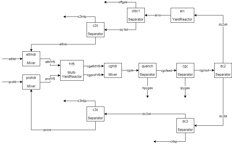
The plant has five reactors called furnaces and named F-1 through F-5, operating in parallel. It has two feed streams: ethane and propane. The fresh feeds are mixed with recycle streams and fed to the furnaces. The cracked gas leaving the furnaces is separated in a series of distillation columns that will be modeled as Separator blocks. A StoicReactor block is used to model the acetylene reactors, which are a series of plug flow reactors that catalytically convert acetylene into ethylene and ethane.
m = Model("ethylene_plant", "index", us)
fs = m.index_fs
The ethane and propane feed streams each contain only one component:
c_ethfeed = {"c2h6"}
c_profeed = {"c3h8"}
The fresh feed streams are mixed with ethane and propane recycle streams. The component lists for the recycle streams are:
c_ethrec = {"c2h4", "c2h6"}
c_prorec = {"c3h6", "c3h8", "mapd"}
The fresh feed streams are mixed with their recycle streams in Mixer blocks:
ethfd, ethre, ethf1f5, profd, prore, prof1f5 = fs:Streams(
        {"ethfd"   , c_ethfeed},   -- Ethane fresh feed
        {"ethre"   , c_ethrec },   -- Ethane recycle
        {"ethf1f5" , c_ethrec },   -- Mixed fresh ethane feed and ethane recycle to furnaces F-1 through F-5.
        {"profd"   , c_profeed},   -- Propane fresh feed
        {"prore"   , c_prorec },   -- Propane recycle
        {"prof1f5" , c_prorec }    -- Mixed fresh propane feed and propane recycle to furnaces F-1 through F-5.
)

ethhdr = fs:Mixer("ethhdr", {ethfd, ethre}, {ethf1f5})    -- ethane header
prohdr = fs:Mixer("prohdr", {profd, prore}, {prof1f5})    -- propane header

m:show_variables()
┌─────┬────────────────────────────────┬───┬──────────────┬──────────────┬──────────────┬────────┐
│Index│              Name              │Fix│     Value    │     Lower    │     Upper    │  Unit  │
├─────┼────────────────────────────────┼───┼──────────────┼──────────────┼──────────────┼────────┤
│    0│ethhdr.ethfd.mass               │   │             0│              │              │kg/hr   │
│    1│ethhdr.ethfd.mass_c2h6          │ = │             0│              │              │kg/hr   │
│    2│ethhdr.ethfd.massfrac_c2h6      │   │             0│              │              │massfrac│
│    3│ethhdr.ethre.mass               │   │             0│              │              │kg/hr   │
│    4│ethhdr.ethre.mass_c2h4          │ = │             0│              │              │kg/hr   │
│    5│ethhdr.ethre.mass_c2h6          │ = │             0│              │              │kg/hr   │
│    6│ethhdr.ethre.massfrac_c2h4      │   │             0│              │              │massfrac│
│    7│ethhdr.ethre.massfrac_c2h6      │   │             0│              │              │massfrac│
│    8│ethhdr.ethf1f5.mass             │   │             0│              │              │kg/hr   │
│    9│ethhdr.ethf1f5.mass_c2h4        │   │             0│              │              │kg/hr   │
│   10│ethhdr.ethf1f5.mass_c2h6        │   │             0│              │              │kg/hr   │
│   11│ethhdr.ethf1f5.massfrac_c2h4    │   │             0│              │              │massfrac│
│   12│ethhdr.ethf1f5.massfrac_c2h6    │   │             0│              │              │massfrac│
│   13│prohdr.profd.mass               │   │             0│              │              │kg/hr   │
│   14│prohdr.profd.mass_c3h8          │ = │             0│              │              │kg/hr   │
│   15│prohdr.profd.massfrac_c3h8      │   │             0│              │              │massfrac│
│   16│prohdr.prore.mass               │   │             0│              │              │kg/hr   │
│   17│prohdr.prore.mass_c3h6          │ = │             0│              │              │kg/hr   │
│   18│prohdr.prore.mass_c3h8          │ = │             0│              │              │kg/hr   │
│   19│prohdr.prore.mass_mapd          │ = │             0│              │              │kg/hr   │
│   20│prohdr.prore.massfrac_c3h6      │   │             0│              │              │massfrac│
│   21│prohdr.prore.massfrac_c3h8      │   │             0│              │              │massfrac│
│   22│prohdr.prore.massfrac_mapd      │   │             0│              │              │massfrac│
│   23│prohdr.prof1f5.mass             │   │             0│              │              │kg/hr   │
│   24│prohdr.prof1f5.mass_c3h6        │   │             0│              │              │kg/hr   │
│   25│prohdr.prof1f5.mass_c3h8        │   │             0│              │              │kg/hr   │
│   26│prohdr.prof1f5.mass_mapd        │   │             0│              │              │kg/hr   │
│   27│prohdr.prof1f5.massfrac_c3h6    │   │             0│              │              │massfrac│
│   28│prohdr.prof1f5.massfrac_c3h8    │   │             0│              │              │massfrac│
│   29│prohdr.prof1f5.massfrac_mapd    │   │             0│              │              │massfrac│
└─────┴────────────────────────────────┴───┴──────────────┴──────────────┴──────────────┴────────┘
30 Variables shown
The feed and recycle stream component mass flow rates are fixed variables. Their values must be set before the blocks are initialized:
m:eval([[
    ethhdr.ethfd.mass_c2h6 = 80000.0
    prohdr.profd.mass_c3h8 = 34000.0
    ethhdr.ethre.mass_c2h6 = 38805.0
    ethhdr.ethre.mass_c2h4 =   195.0
    prohdr.prore.mass_c3h8 =  4800.0
    prohdr.prore.mass_c3h6 =    25.0
    prohdr.prore.mass_mapd =   175.0
]])
m:init()
m:show_variables()
┌─────┬────────────────────────────────┬───┬──────────────┬──────────────┬──────────────┬────────┐
│Index│              Name              │Fix│     Value    │     Lower    │     Upper    │  Unit  │
├─────┼────────────────────────────────┼───┼──────────────┼──────────────┼──────────────┼────────┤
│    0│ethhdr.ethfd.mass               │   │         80000│              │              │kg/hr   │
│    1│ethhdr.ethfd.mass_c2h6          │ = │         80000│              │              │kg/hr   │
│    2│ethhdr.ethfd.massfrac_c2h6      │   │             1│              │              │massfrac│
│    3│ethhdr.ethre.mass               │   │         39000│              │              │kg/hr   │
│    4│ethhdr.ethre.mass_c2h4          │ = │           195│              │              │kg/hr   │
│    5│ethhdr.ethre.mass_c2h6          │ = │         38805│              │              │kg/hr   │
│    6│ethhdr.ethre.massfrac_c2h4      │   │         0.005│              │              │massfrac│
│    7│ethhdr.ethre.massfrac_c2h6      │   │         0.995│              │              │massfrac│
│    8│ethhdr.ethf1f5.mass             │   │        119000│              │              │kg/hr   │
│    9│ethhdr.ethf1f5.mass_c2h4        │   │           195│              │              │kg/hr   │
│   10│ethhdr.ethf1f5.mass_c2h6        │   │        118805│              │              │kg/hr   │
│   11│ethhdr.ethf1f5.massfrac_c2h4    │   │   0.001638655│              │              │massfrac│
│   12│ethhdr.ethf1f5.massfrac_c2h6    │   │     0.9983613│              │              │massfrac│
│   13│prohdr.profd.mass               │   │         34000│              │              │kg/hr   │
│   14│prohdr.profd.mass_c3h8          │ = │         34000│              │              │kg/hr   │
│   15│prohdr.profd.massfrac_c3h8      │   │             1│              │              │massfrac│
│   16│prohdr.prore.mass               │   │          5000│              │              │kg/hr   │
│   17│prohdr.prore.mass_c3h6          │ = │            25│              │              │kg/hr   │
│   18│prohdr.prore.mass_c3h8          │ = │          4800│              │              │kg/hr   │
│   19│prohdr.prore.mass_mapd          │ = │           175│              │              │kg/hr   │
│   20│prohdr.prore.massfrac_c3h6      │   │         0.005│              │              │massfrac│
│   21│prohdr.prore.massfrac_c3h8      │   │          0.96│              │              │massfrac│
│   22│prohdr.prore.massfrac_mapd      │   │         0.035│              │              │massfrac│
│   23│prohdr.prof1f5.mass             │   │         39000│              │              │kg/hr   │
│   24│prohdr.prof1f5.mass_c3h6        │   │            25│              │              │kg/hr   │
│   25│prohdr.prof1f5.mass_c3h8        │   │         38800│              │              │kg/hr   │
│   26│prohdr.prof1f5.mass_mapd        │   │           175│              │              │kg/hr   │
│   27│prohdr.prof1f5.massfrac_c3h6    │   │  0.0006410256│              │              │massfrac│
│   28│prohdr.prof1f5.massfrac_c3h8    │   │     0.9948718│              │              │massfrac│
│   29│prohdr.prof1f5.massfrac_mapd    │   │   0.004487179│              │              │massfrac│
└─────┴────────────────────────────────┴───┴──────────────┴──────────────┴──────────────┴────────┘
30 Variables shown
We'll fix the total mass flow rates of the two feed streams and free the component mass flow rates:
m:eval([[
    free ethhdr.ethfd.mass_c2h6
    fix  ethhdr.ethfd.mass
    free prohdr.profd.mass_c3h8
    fix  prohdr.profd.mass
]])
print(m)
Model: ethylene_plant
  Number of equations          = 23
  Number of free variables     = 23
  Number of fixed variables    = 7
  Number of variables          = 30
  Number of Jacobian non-zeros = 66
  Number of Hessian non-zeros  = 12
Model is square
We solve the model:
sv:solve(m)
This is Ipopt version 3.14.19, running with linear solver MUMPS 5.6.2.

Number of nonzeros in equality constraint Jacobian...:       47
Number of nonzeros in inequality constraint Jacobian.:        0
Number of nonzeros in Lagrangian Hessian.............:       10

Total number of variables............................:       23
                     variables with only lower bounds:        0
                variables with lower and upper bounds:        0
                     variables with only upper bounds:        0
Total number of equality constraints.................:       23
Total number of inequality constraints...............:        0
        inequality constraints with only lower bounds:        0
   inequality constraints with lower and upper bounds:        0
        inequality constraints with only upper bounds:        0

iter    objective    inf_pr   inf_du lg(mu)  ||d||  lg(rg) alpha_du alpha_pr  ls
   0  1.0000000e+00 1.95e-12 0.00e+00  -1.0 0.00e+00    -  0.00e+00 0.00e+00   0

Number of Iterations....: 0

                                   (scaled)                 (unscaled)
Objective...............:  -1.0000000000000000e+00    1.0000000000000000e+00
Dual infeasibility......:   0.0000000000000000e+00    0.0000000000000000e+00
Constraint violation....:   3.5527136788005009e-15    1.9495516312417749e-12
Variable bound violation:   0.0000000000000000e+00    0.0000000000000000e+00
Complementarity.........:   0.0000000000000000e+00    0.0000000000000000e+00
Overall NLP error.......:   3.5527136788005009e-15    1.9495516312417749e-12


Number of objective function evaluations             = 1
Number of objective gradient evaluations             = 1
Number of equality constraint evaluations            = 1
Number of inequality constraint evaluations          = 0
Number of equality constraint Jacobian evaluations   = 1
Number of inequality constraint Jacobian evaluations = 0
Number of Lagrangian Hessian evaluations             = 0
Total seconds in IPOPT                               = 0.000

EXIT: Optimal Solution Found.
0
The furnaces will be modelled with a MultiYieldReactor that has two feeds named eth and pro and produces two cracked gas outlet streams, one for each feed. The cracked gas components are:
c_cg = {"h2", "ch4", "c2h2", "c2h4", "c2h6", "c3h6", "c3h8", "mapd", "c4s", "pygas"}
The cracked gas streams are:
cgethf1f5, cgprof1f5 = fs:Streams(
    {"cgethf1f5" , c_cg},
    {"cgprof1f5" , c_cg}
)
We can create the MultiYieldReactor block and connect its inlet streams. The furnaces will be named furn:
f1f5 = fs:MultiYieldReactor("f1f5", {ethf1f5, prof1f5}, {cgethf1f5, cgprof1f5}, "furn", "eth", "pro")
f1f5:connect()       -- connect the inlet streams
f1f5:show_fixed()    -- show only the fixed variables in f1f5
┌─────┬────────────────────────────────┬───┬──────────────┬──────────────┬──────────────┬────────┐
│Index│              Name              │Fix│     Value    │     Lower    │     Upper    │  Unit  │
├─────┼────────────────────────────────┼───┼──────────────┼──────────────┼──────────────┼────────┤
│   84│f1f5.eth_y_h2_from_c2h4         │ = │             0│              │              │frac    │
│   85│f1f5.eth_y_ch4_from_c2h4        │ = │             0│              │              │frac    │
│   86│f1f5.eth_y_c2h2_from_c2h4       │ = │             0│              │              │frac    │
│   88│f1f5.eth_y_c2h6_from_c2h4       │ = │             0│              │              │frac    │
│   89│f1f5.eth_y_c3h6_from_c2h4       │ = │             0│              │              │frac    │
│   90│f1f5.eth_y_c3h8_from_c2h4       │ = │             0│              │              │frac    │
│   91│f1f5.eth_y_mapd_from_c2h4       │ = │             0│              │              │frac    │
│   92│f1f5.eth_y_c4s_from_c2h4        │ = │             0│              │              │frac    │
│   93│f1f5.eth_y_pygas_from_c2h4      │ = │             0│              │              │frac    │
│   94│f1f5.eth_y_h2_from_c2h6         │ = │             0│              │              │frac    │
│   95│f1f5.eth_y_ch4_from_c2h6        │ = │             0│              │              │frac    │
│   96│f1f5.eth_y_c2h2_from_c2h6       │ = │             0│              │              │frac    │
│   97│f1f5.eth_y_c2h4_from_c2h6       │ = │             0│              │              │frac    │
│   99│f1f5.eth_y_c3h6_from_c2h6       │ = │             0│              │              │frac    │
│  100│f1f5.eth_y_c3h8_from_c2h6       │ = │             0│              │              │frac    │
│  101│f1f5.eth_y_mapd_from_c2h6       │ = │             0│              │              │frac    │
│  102│f1f5.eth_y_c4s_from_c2h6        │ = │             0│              │              │frac    │
│  103│f1f5.eth_y_pygas_from_c2h6      │ = │             0│              │              │frac    │
│  104│f1f5.pro_y_h2_from_c3h6         │ = │             0│              │              │frac    │
│  105│f1f5.pro_y_ch4_from_c3h6        │ = │             0│              │              │frac    │
│  106│f1f5.pro_y_c2h2_from_c3h6       │ = │             0│              │              │frac    │
│  107│f1f5.pro_y_c2h4_from_c3h6       │ = │             0│              │              │frac    │
│  108│f1f5.pro_y_c2h6_from_c3h6       │ = │             0│              │              │frac    │
│  110│f1f5.pro_y_c3h8_from_c3h6       │ = │             0│              │              │frac    │
│  111│f1f5.pro_y_mapd_from_c3h6       │ = │             0│              │              │frac    │
│  112│f1f5.pro_y_c4s_from_c3h6        │ = │             0│              │              │frac    │
│  113│f1f5.pro_y_pygas_from_c3h6      │ = │             0│              │              │frac    │
│  114│f1f5.pro_y_h2_from_c3h8         │ = │             0│              │              │frac    │
│  115│f1f5.pro_y_ch4_from_c3h8        │ = │             0│              │              │frac    │
│  116│f1f5.pro_y_c2h2_from_c3h8       │ = │             0│              │              │frac    │
│  117│f1f5.pro_y_c2h4_from_c3h8       │ = │             0│              │              │frac    │
│  118│f1f5.pro_y_c2h6_from_c3h8       │ = │             0│              │              │frac    │
│  119│f1f5.pro_y_c3h6_from_c3h8       │ = │             0│              │              │frac    │
│  121│f1f5.pro_y_mapd_from_c3h8       │ = │             0│              │              │frac    │
│  122│f1f5.pro_y_c4s_from_c3h8        │ = │             0│              │              │frac    │
│  123│f1f5.pro_y_pygas_from_c3h8      │ = │             0│              │              │frac    │
│  124│f1f5.pro_y_h2_from_mapd         │ = │             0│              │              │frac    │
│  125│f1f5.pro_y_ch4_from_mapd        │ = │             0│              │              │frac    │
│  126│f1f5.pro_y_c2h2_from_mapd       │ = │             0│              │              │frac    │
│  127│f1f5.pro_y_c2h4_from_mapd       │ = │             0│              │              │frac    │
│  128│f1f5.pro_y_c2h6_from_mapd       │ = │             0│              │              │frac    │
│  129│f1f5.pro_y_c3h6_from_mapd       │ = │             0│              │              │frac    │
│  130│f1f5.pro_y_c3h8_from_mapd       │ = │             0│              │              │frac    │
│  132│f1f5.pro_y_c4s_from_mapd        │ = │             0│              │              │frac    │
│  133│f1f5.pro_y_pygas_from_mapd      │ = │             0│              │              │frac    │
│  136│f1f5.eth_feed_rate              │ = │             0│              │              │kg/hr   │
│  138│f1f5.pro_feed_rate              │ = │             0│              │              │kg/hr   │
└─────┴────────────────────────────────┴───┴──────────────┴──────────────┴──────────────┴────────┘
47 Variables shown
We set the values of all the fixed variables by reading them from a file:
m:eval(read_vars("f1f5_init.lua"))
f1f5:show_fixed()
┌─────┬────────────────────────────────┬───┬──────────────┬──────────────┬──────────────┬────────┐
│Index│              Name              │Fix│     Value    │     Lower    │     Upper    │  Unit  │
├─────┼────────────────────────────────┼───┼──────────────┼──────────────┼──────────────┼────────┤
│   84│f1f5.eth_y_h2_from_c2h4         │ = │        -0.009│              │              │frac    │
│   85│f1f5.eth_y_ch4_from_c2h4        │ = │         0.129│              │              │frac    │
│   86│f1f5.eth_y_c2h2_from_c2h4       │ = │         0.004│              │              │frac    │
│   88│f1f5.eth_y_c2h6_from_c2h4       │ = │             0│              │              │frac    │
│   89│f1f5.eth_y_c3h6_from_c2h4       │ = │         0.003│              │              │frac    │
│   90│f1f5.eth_y_c3h8_from_c2h4       │ = │         0.002│              │              │frac    │
│   91│f1f5.eth_y_mapd_from_c2h4       │ = │             0│              │              │frac    │
│   92│f1f5.eth_y_c4s_from_c2h4        │ = │          0.05│              │              │frac    │
│   93│f1f5.eth_y_pygas_from_c2h4      │ = │          0.15│              │              │frac    │
│   94│f1f5.eth_y_h2_from_c2h6         │ = │        0.0411│              │              │frac    │
│   95│f1f5.eth_y_ch4_from_c2h6        │ = │          0.05│              │              │frac    │
│   96│f1f5.eth_y_c2h2_from_c2h6       │ = │         0.003│              │              │frac    │
│   97│f1f5.eth_y_c2h4_from_c2h6       │ = │         0.495│              │              │frac    │
│   99│f1f5.eth_y_c3h6_from_c2h6       │ = │        0.0043│              │              │frac    │
│  100│f1f5.eth_y_c3h8_from_c2h6       │ = │          0.01│              │              │frac    │
│  101│f1f5.eth_y_mapd_from_c2h6       │ = │        0.0002│              │              │frac    │
│  102│f1f5.eth_y_c4s_from_c2h6        │ = │          0.03│              │              │frac    │
│  103│f1f5.eth_y_pygas_from_c2h6      │ = │          0.02│              │              │frac    │
│  104│f1f5.pro_y_h2_from_c3h6         │ = │       -0.0035│              │              │frac    │
│  105│f1f5.pro_y_ch4_from_c3h6        │ = │          0.15│              │              │frac    │
│  106│f1f5.pro_y_c2h2_from_c3h6       │ = │         0.005│              │              │frac    │
│  107│f1f5.pro_y_c2h4_from_c3h6       │ = │          0.04│              │              │frac    │
│  108│f1f5.pro_y_c2h6_from_c3h6       │ = │         0.004│              │              │frac    │
│  110│f1f5.pro_y_c3h8_from_c3h6       │ = │             0│              │              │frac    │
│  111│f1f5.pro_y_mapd_from_c3h6       │ = │         0.002│              │              │frac    │
│  112│f1f5.pro_y_c4s_from_c3h6        │ = │          0.03│              │              │frac    │
│  113│f1f5.pro_y_pygas_from_c3h6      │ = │          0.15│              │              │frac    │
│  114│f1f5.pro_y_h2_from_c3h8         │ = │          0.01│              │              │frac    │
│  115│f1f5.pro_y_ch4_from_c3h8        │ = │          0.21│              │              │frac    │
│  116│f1f5.pro_y_c2h2_from_c3h8       │ = │         0.004│              │              │frac    │
│  117│f1f5.pro_y_c2h4_from_c3h8       │ = │          0.35│              │              │frac    │
│  118│f1f5.pro_y_c2h6_from_c3h8       │ = │          0.04│              │              │frac    │
│  119│f1f5.pro_y_c3h6_from_c3h8       │ = │          0.16│              │              │frac    │
│  121│f1f5.pro_y_mapd_from_c3h8       │ = │         0.004│              │              │frac    │
│  122│f1f5.pro_y_c4s_from_c3h8        │ = │         0.015│              │              │frac    │
│  123│f1f5.pro_y_pygas_from_c3h8      │ = │         0.025│              │              │frac    │
│  124│f1f5.pro_y_h2_from_mapd         │ = │             0│              │              │frac    │
│  125│f1f5.pro_y_ch4_from_mapd        │ = │             0│              │              │frac    │
│  126│f1f5.pro_y_c2h2_from_mapd       │ = │             0│              │              │frac    │
│  127│f1f5.pro_y_c2h4_from_mapd       │ = │             0│              │              │frac    │
│  128│f1f5.pro_y_c2h6_from_mapd       │ = │             0│              │              │frac    │
│  129│f1f5.pro_y_c3h6_from_mapd       │ = │             1│              │              │frac    │
│  130│f1f5.pro_y_c3h8_from_mapd       │ = │             0│              │              │frac    │
│  132│f1f5.pro_y_c4s_from_mapd        │ = │             0│              │              │frac    │
│  133│f1f5.pro_y_pygas_from_mapd      │ = │             0│              │              │frac    │
│  136│f1f5.eth_feed_rate              │ = │         30000│              │              │kg/hr   │
│  138│f1f5.pro_feed_rate              │ = │         40000│              │              │kg/hr   │
└─────┴────────────────────────────────┴───┴──────────────┴──────────────┴──────────────┴────────┘
47 Variables shown
Initialize f1f5 and solve the model:
f1f5:init()
sv:solve(m)
f1f5:show_variables()
This is Ipopt version 3.14.19, running with linear solver MUMPS 5.6.2.
Number of nonzeros in equality constraint Jacobian...: 251
Number of nonzeros in inequality constraint Jacobian.: 0
Number of nonzeros in Lagrangian Hessian.............: 40
Total number of variables............................: 86
variables with only lower bounds: 0
variables with lower and upper bounds: 0
variables with only upper bounds: 0
Total number of equality constraints.................: 86
Total number of inequality constraints...............: 0
inequality constraints with only lower bounds: 0
inequality constraints with lower and upper bounds: 0
inequality constraints with only upper bounds: 0
iter objective inf_pr inf_du lg(mu) ||d|| lg(rg) alpha_du alpha_pr ls
0 1.0000000e+00 3.55e-12 0.00e+00 -1.0 0.00e+00 - 0.00e+00 0.00e+00 0
Number of Iterations....: 0
(scaled) (unscaled)
Objective...............: -1.0000000000000000e+00 1.0000000000000000e+00
Dual infeasibility......: 0.0000000000000000e+00 0.0000000000000000e+00
Constraint violation....: 9.0949470177292824e-13 3.5527136788005009e-12
Variable bound violation: 0.0000000000000000e+00 0.0000000000000000e+00
Complementarity.........: 0.0000000000000000e+00 0.0000000000000000e+00
Overall NLP error.......: 9.0949470177292824e-13 3.5527136788005009e-12
Number of objective function evaluations = 1
Number of objective gradient evaluations = 1
Number of equality constraint evaluations = 1
Number of inequality constraint evaluations = 0
Number of equality constraint Jacobian evaluations = 1
Number of inequality constraint Jacobian evaluations = 0
Number of Lagrangian Hessian evaluations = 0
Total seconds in IPOPT = 0.001
EXIT: Optimal Solution Found.
┌─────┬────────────────────────────────┬───┬──────────────┬──────────────┬──────────────┬────────┐
│Index│ Name │Fix│ Value │ Lower │ Upper │ Unit │
├─────┼────────────────────────────────┼───┼──────────────┼──────────────┼──────────────┼────────┤
│ 30│f1f5.ethf1f5.mass │ │ 119000│ │ │kg/hr │
│ 31│f1f5.ethf1f5.mass_c2h4 │ │ 195│ │ │kg/hr │
│ 32│f1f5.ethf1f5.mass_c2h6 │ │ 118805│ │ │kg/hr │
│ 33│f1f5.ethf1f5.massfrac_c2h4 │ │ 0.001638655│ │ │massfrac│
│ 34│f1f5.ethf1f5.massfrac_c2h6 │ │ 0.9983613│ │ │massfrac│
│ 35│f1f5.prof1f5.mass │ │ 39000│ │ │kg/hr │
│ 36│f1f5.prof1f5.mass_c3h6 │ │ 25│ │ │kg/hr │
│ 37│f1f5.prof1f5.mass_c3h8 │ │ 38800│ │ │kg/hr │
│ 38│f1f5.prof1f5.mass_mapd │ │ 175│ │ │kg/hr │
│ 39│f1f5.prof1f5.massfrac_c3h6 │ │ 0.0006410256│ │ │massfrac│
│ 40│f1f5.prof1f5.massfrac_c3h8 │ │ 0.9948718│ │ │massfrac│
│ 41│f1f5.prof1f5.massfrac_mapd │ │ 0.004487179│ │ │massfrac│
│ 42│f1f5.cgethf1f5.mass │ │ 119000│ │ │kg/hr │
│ 43│f1f5.cgethf1f5.mass_h2 │ │ 4881.13│ │ │kg/hr │
│ 44│f1f5.cgethf1f5.mass_ch4 │ │ 5965.405│ │ │kg/hr │
│ 45│f1f5.cgethf1f5.mass_c2h2 │ │ 357.195│ │ │kg/hr │
│ 46│f1f5.cgethf1f5.mass_c2h4 │ │ 58939.32│ │ │kg/hr │
│ 47│f1f5.cgethf1f5.mass_c2h6 │ │ 41154.05│ │ │kg/hr │
│ 48│f1f5.cgethf1f5.mass_c3h6 │ │ 511.4465│ │ │kg/hr │
│ 49│f1f5.cgethf1f5.mass_c3h8 │ │ 1188.44│ │ │kg/hr │
│ 50│f1f5.cgethf1f5.mass_mapd │ │ 23.761│ │ │kg/hr │
│ 51│f1f5.cgethf1f5.mass_c4s │ │ 3573.9│ │ │kg/hr │
│ 52│f1f5.cgethf1f5.mass_pygas │ │ 2405.35│ │ │kg/hr │
│ 53│f1f5.cgethf1f5.massfrac_h2 │ │ 0.0410179│ │ │massfrac│
│ 54│f1f5.cgethf1f5.massfrac_ch4 │ │ 0.05012945│ │ │massfrac│
│ 55│f1f5.cgethf1f5.massfrac_c2h2 │ │ 0.003001639│ │ │massfrac│
│ 56│f1f5.cgethf1f5.massfrac_c2h4 │ │ 0.4952884│ │ │massfrac│
│ 57│f1f5.cgethf1f5.massfrac_c2h6 │ │ 0.3458324│ │ │massfrac│
│ 58│f1f5.cgethf1f5.massfrac_c3h6 │ │ 0.00429787│ │ │massfrac│
│ 59│f1f5.cgethf1f5.massfrac_c3h8 │ │ 0.009986891│ │ │massfrac│
│ 60│f1f5.cgethf1f5.massfrac_mapd │ │ 0.0001996723│ │ │massfrac│
│ 61│f1f5.cgethf1f5.massfrac_c4s │ │ 0.03003277│ │ │massfrac│
│ 62│f1f5.cgethf1f5.massfrac_pygas │ │ 0.02021303│ │ │massfrac│
│ 63│f1f5.cgprof1f5.mass │ │ 39000│ │ │kg/hr │
│ 64│f1f5.cgprof1f5.mass_h2 │ │ 387.9125│ │ │kg/hr │
│ 65│f1f5.cgprof1f5.mass_ch4 │ │ 8151.75│ │ │kg/hr │
│ 66│f1f5.cgprof1f5.mass_c2h2 │ │ 155.325│ │ │kg/hr │
│ 67│f1f5.cgprof1f5.mass_c2h4 │ │ 13581│ │ │kg/hr │
│ 68│f1f5.cgprof1f5.mass_c2h6 │ │ 1552.1│ │ │kg/hr │
│ 69│f1f5.cgprof1f5.mass_c3h6 │ │ 6398.562│ │ │kg/hr │
│ 70│f1f5.cgprof1f5.mass_c3h8 │ │ 7061.6│ │ │kg/hr │
│ 71│f1f5.cgprof1f5.mass_mapd │ │ 155.25│ │ │kg/hr │
│ 72│f1f5.cgprof1f5.mass_c4s │ │ 582.75│ │ │kg/hr │
│ 73│f1f5.cgprof1f5.mass_pygas │ │ 973.75│ │ │kg/hr │
│ 74│f1f5.cgprof1f5.massfrac_h2 │ │ 0.009946474│ │ │massfrac│
│ 75│f1f5.cgprof1f5.massfrac_ch4 │ │ 0.2090192│ │ │massfrac│
│ 76│f1f5.cgprof1f5.massfrac_c2h2 │ │ 0.003982692│ │ │massfrac│
│ 77│f1f5.cgprof1f5.massfrac_c2h4 │ │ 0.3482308│ │ │massfrac│
│ 78│f1f5.cgprof1f5.massfrac_c2h6 │ │ 0.03979744│ │ │massfrac│
│ 79│f1f5.cgprof1f5.massfrac_c3h6 │ │ 0.1640657│ │ │massfrac│
│ 80│f1f5.cgprof1f5.massfrac_c3h8 │ │ 0.1810667│ │ │massfrac│
│ 81│f1f5.cgprof1f5.massfrac_mapd │ │ 0.003980769│ │ │massfrac│
│ 82│f1f5.cgprof1f5.massfrac_c4s │ │ 0.01494231│ │ │massfrac│
│ 83│f1f5.cgprof1f5.massfrac_pygas │ │ 0.02496795│ │ │massfrac│
│ 84│f1f5.eth_y_h2_from_c2h4 │ = │ -0.009│ │ │frac │
│ 85│f1f5.eth_y_ch4_from_c2h4 │ = │ 0.129│ │ │frac │
│ 86│f1f5.eth_y_c2h2_from_c2h4 │ = │ 0.004│ │ │frac │
│ 87│f1f5.eth_y_c2h4_from_c2h4 │ │ 0.671│ │ │frac │
│ 88│f1f5.eth_y_c2h6_from_c2h4 │ = │ 0│ │ │frac │
│ 89│f1f5.eth_y_c3h6_from_c2h4 │ = │ 0.003│ │ │frac │
│ 90│f1f5.eth_y_c3h8_from_c2h4 │ = │ 0.002│ │ │frac │
│ 91│f1f5.eth_y_mapd_from_c2h4 │ = │ 0│ │ │frac │
│ 92│f1f5.eth_y_c4s_from_c2h4 │ = │ 0.05│ │ │frac │
│ 93│f1f5.eth_y_pygas_from_c2h4 │ = │ 0.15│ │ │frac │
│ 94│f1f5.eth_y_h2_from_c2h6 │ = │ 0.0411│ │ │frac │
│ 95│f1f5.eth_y_ch4_from_c2h6 │ = │ 0.05│ │ │frac │
│ 96│f1f5.eth_y_c2h2_from_c2h6 │ = │ 0.003│ │ │frac │
│ 97│f1f5.eth_y_c2h4_from_c2h6 │ = │ 0.495│ │ │frac │
│ 98│f1f5.eth_y_c2h6_from_c2h6 │ │ 0.3464│ │ │frac │
│ 99│f1f5.eth_y_c3h6_from_c2h6 │ = │ 0.0043│ │ │frac │
│ 100│f1f5.eth_y_c3h8_from_c2h6 │ = │ 0.01│ │ │frac │
│ 101│f1f5.eth_y_mapd_from_c2h6 │ = │ 0.0002│ │ │frac │
│ 102│f1f5.eth_y_c4s_from_c2h6 │ = │ 0.03│ │ │frac │
│ 103│f1f5.eth_y_pygas_from_c2h6 │ = │ 0.02│ │ │frac │
│ 104│f1f5.pro_y_h2_from_c3h6 │ = │ -0.0035│ │ │frac │
│ 105│f1f5.pro_y_ch4_from_c3h6 │ = │ 0.15│ │ │frac │
│ 106│f1f5.pro_y_c2h2_from_c3h6 │ = │ 0.005│ │ │frac │
│ 107│f1f5.pro_y_c2h4_from_c3h6 │ = │ 0.04│ │ │frac │
│ 108│f1f5.pro_y_c2h6_from_c3h6 │ = │ 0.004│ │ │frac │
│ 109│f1f5.pro_y_c3h6_from_c3h6 │ │ 0.6225│ │ │frac │
│ 110│f1f5.pro_y_c3h8_from_c3h6 │ = │ 0│ │ │frac │
│ 111│f1f5.pro_y_mapd_from_c3h6 │ = │ 0.002│ │ │frac │
│ 112│f1f5.pro_y_c4s_from_c3h6 │ = │ 0.03│ │ │frac │
│ 113│f1f5.pro_y_pygas_from_c3h6 │ = │ 0.15│ │ │frac │
│ 114│f1f5.pro_y_h2_from_c3h8 │ = │ 0.01│ │ │frac │
│ 115│f1f5.pro_y_ch4_from_c3h8 │ = │ 0.21│ │ │frac │
│ 116│f1f5.pro_y_c2h2_from_c3h8 │ = │ 0.004│ │ │frac │
│ 117│f1f5.pro_y_c2h4_from_c3h8 │ = │ 0.35│ │ │frac │
│ 118│f1f5.pro_y_c2h6_from_c3h8 │ = │ 0.04│ │ │frac │
│ 119│f1f5.pro_y_c3h6_from_c3h8 │ = │ 0.16│ │ │frac │
│ 120│f1f5.pro_y_c3h8_from_c3h8 │ │ 0.182│ │ │frac │
│ 121│f1f5.pro_y_mapd_from_c3h8 │ = │ 0.004│ │ │frac │
│ 122│f1f5.pro_y_c4s_from_c3h8 │ = │ 0.015│ │ │frac │
│ 123│f1f5.pro_y_pygas_from_c3h8 │ = │ 0.025│ │ │frac │
│ 124│f1f5.pro_y_h2_from_mapd │ = │ 0│ │ │frac │
│ 125│f1f5.pro_y_ch4_from_mapd │ = │ 0│ │ │frac │
│ 126│f1f5.pro_y_c2h2_from_mapd │ = │ 0│ │ │frac │
│ 127│f1f5.pro_y_c2h4_from_mapd │ = │ 0│ │ │frac │
│ 128│f1f5.pro_y_c2h6_from_mapd │ = │ 0│ │ │frac │
│ 129│f1f5.pro_y_c3h6_from_mapd │ = │ 1│ │ │frac │
│ 130│f1f5.pro_y_c3h8_from_mapd │ = │ 0│ │ │frac │
│ 131│f1f5.pro_y_mapd_from_mapd │ │ 0│ │ │frac │
│ 132│f1f5.pro_y_c4s_from_mapd │ = │ 0│ │ │frac │
│ 133│f1f5.pro_y_pygas_from_mapd │ = │ 0│ │ │frac │
│ 134│f1f5.total_feed_mass │ │ 158000│ │ │kg/hr │
│ 135│f1f5.eth_n_furn │ │ 3.966667│ │ │# │
│ 136│f1f5.eth_feed_rate │ = │ 30000│ │ │kg/hr │
│ 137│f1f5.pro_n_furn │ │ 0.975│ │ │# │
│ 138│f1f5.pro_feed_rate │ = │ 40000│ │ │kg/hr │
│ 139│f1f5.n_furn │ │ 4.941667│ │ │# │
└─────┴────────────────────────────────┴───┴──────────────┴──────────────┴──────────────┴────────┘
110 Variables shown
The cracked gas streams leaving the furnaces are mixed together in the cracked gas header. The same pattern is used to add additional blocks to the model:
- Define component groups
- Create inlet and outlet streams
- Create the block
- Connect the block's inlet streams to the outlet streams of upstream blocks
- Configure variable specifications if necessary
- Set values of the fixed variables
- Initialize the new block
- Solve the model and show variables if desired
To keep the output concise we'll avoid solving the model repeatedly in this example. In practice, a solve is usually done after adding each new block.
-- Cracked gas header.
cgas = fs:Streams( {"cgas", c_cg} )
cghdr = fs:Mixer("cghdr", {cgethf1f5, cgprof1f5}, {cgas})
cghdr:connect()
cghdr:init()
cghdr:show_vars()
┌─────┬────────────────────────────────┬───┬──────────────┬──────────────┬──────────────┬────────┐
│Index│              Name              │Fix│     Value    │     Lower    │     Upper    │  Unit  │
├─────┼────────────────────────────────┼───┼──────────────┼──────────────┼──────────────┼────────┤
│  140│cghdr.cgethf1f5.mass            │   │        119000│              │              │kg/hr   │
│  141│cghdr.cgethf1f5.mass_h2         │   │       4881.13│              │              │kg/hr   │
│  142│cghdr.cgethf1f5.mass_ch4        │   │      5965.405│              │              │kg/hr   │
│  143│cghdr.cgethf1f5.mass_c2h2       │   │       357.195│              │              │kg/hr   │
│  144│cghdr.cgethf1f5.mass_c2h4       │   │      58939.32│              │              │kg/hr   │
│  145│cghdr.cgethf1f5.mass_c2h6       │   │      41154.05│              │              │kg/hr   │
│  146│cghdr.cgethf1f5.mass_c3h6       │   │      511.4465│              │              │kg/hr   │
│  147│cghdr.cgethf1f5.mass_c3h8       │   │       1188.44│              │              │kg/hr   │
│  148│cghdr.cgethf1f5.mass_mapd       │   │        23.761│              │              │kg/hr   │
│  149│cghdr.cgethf1f5.mass_c4s        │   │        3573.9│              │              │kg/hr   │
│  150│cghdr.cgethf1f5.mass_pygas      │   │       2405.35│              │              │kg/hr   │
│  151│cghdr.cgethf1f5.massfrac_h2     │   │     0.0410179│              │              │massfrac│
│  152│cghdr.cgethf1f5.massfrac_ch4    │   │    0.05012945│              │              │massfrac│
│  153│cghdr.cgethf1f5.massfrac_c2h2   │   │   0.003001639│              │              │massfrac│
│  154│cghdr.cgethf1f5.massfrac_c2h4   │   │     0.4952884│              │              │massfrac│
│  155│cghdr.cgethf1f5.massfrac_c2h6   │   │     0.3458324│              │              │massfrac│
│  156│cghdr.cgethf1f5.massfrac_c3h6   │   │    0.00429787│              │              │massfrac│
│  157│cghdr.cgethf1f5.massfrac_c3h8   │   │   0.009986891│              │              │massfrac│
│  158│cghdr.cgethf1f5.massfrac_mapd   │   │  0.0001996723│              │              │massfrac│
│  159│cghdr.cgethf1f5.massfrac_c4s    │   │    0.03003277│              │              │massfrac│
│  160│cghdr.cgethf1f5.massfrac_pygas  │   │    0.02021303│              │              │massfrac│
│  161│cghdr.cgprof1f5.mass            │   │         39000│              │              │kg/hr   │
│  162│cghdr.cgprof1f5.mass_h2         │   │      387.9125│              │              │kg/hr   │
│  163│cghdr.cgprof1f5.mass_ch4        │   │       8151.75│              │              │kg/hr   │
│  164│cghdr.cgprof1f5.mass_c2h2       │   │       155.325│              │              │kg/hr   │
│  165│cghdr.cgprof1f5.mass_c2h4       │   │         13581│              │              │kg/hr   │
│  166│cghdr.cgprof1f5.mass_c2h6       │   │        1552.1│              │              │kg/hr   │
│  167│cghdr.cgprof1f5.mass_c3h6       │   │      6398.562│              │              │kg/hr   │
│  168│cghdr.cgprof1f5.mass_c3h8       │   │        7061.6│              │              │kg/hr   │
│  169│cghdr.cgprof1f5.mass_mapd       │   │        155.25│              │              │kg/hr   │
│  170│cghdr.cgprof1f5.mass_c4s        │   │        582.75│              │              │kg/hr   │
│  171│cghdr.cgprof1f5.mass_pygas      │   │        973.75│              │              │kg/hr   │
│  172│cghdr.cgprof1f5.massfrac_h2     │   │   0.009946474│              │              │massfrac│
│  173│cghdr.cgprof1f5.massfrac_ch4    │   │     0.2090192│              │              │massfrac│
│  174│cghdr.cgprof1f5.massfrac_c2h2   │   │   0.003982692│              │              │massfrac│
│  175│cghdr.cgprof1f5.massfrac_c2h4   │   │     0.3482308│              │              │massfrac│
│  176│cghdr.cgprof1f5.massfrac_c2h6   │   │    0.03979744│              │              │massfrac│
│  177│cghdr.cgprof1f5.massfrac_c3h6   │   │     0.1640657│              │              │massfrac│
│  178│cghdr.cgprof1f5.massfrac_c3h8   │   │     0.1810667│              │              │massfrac│
│  179│cghdr.cgprof1f5.massfrac_mapd   │   │   0.003980769│              │              │massfrac│
│  180│cghdr.cgprof1f5.massfrac_c4s    │   │    0.01494231│              │              │massfrac│
│  181│cghdr.cgprof1f5.massfrac_pygas  │   │    0.02496795│              │              │massfrac│
│  182│cghdr.cgas.mass                 │   │        158000│              │              │kg/hr   │
│  183│cghdr.cgas.mass_h2              │   │      5269.043│              │              │kg/hr   │
│  184│cghdr.cgas.mass_ch4             │   │      14117.16│              │              │kg/hr   │
│  185│cghdr.cgas.mass_c2h2            │   │        512.52│              │              │kg/hr   │
│  186│cghdr.cgas.mass_c2h4            │   │      72520.32│              │              │kg/hr   │
│  187│cghdr.cgas.mass_c2h6            │   │      42706.15│              │              │kg/hr   │
│  188│cghdr.cgas.mass_c3h6            │   │      6910.009│              │              │kg/hr   │
│  189│cghdr.cgas.mass_c3h8            │   │       8250.04│              │              │kg/hr   │
│  190│cghdr.cgas.mass_mapd            │   │       179.011│              │              │kg/hr   │
│  191│cghdr.cgas.mass_c4s             │   │       4156.65│              │              │kg/hr   │
│  192│cghdr.cgas.mass_pygas           │   │        3379.1│              │              │kg/hr   │
│  193│cghdr.cgas.massfrac_h2          │   │    0.03334837│              │              │massfrac│
│  194│cghdr.cgas.massfrac_ch4         │   │    0.08934908│              │              │massfrac│
│  195│cghdr.cgas.massfrac_c2h2        │   │   0.003243797│              │              │massfrac│
│  196│cghdr.cgas.massfrac_c2h4        │   │     0.4589894│              │              │massfrac│
│  197│cghdr.cgas.massfrac_c2h6        │   │     0.2702921│              │              │massfrac│
│  198│cghdr.cgas.massfrac_c3h6        │   │    0.04373423│              │              │massfrac│
│  199│cghdr.cgas.massfrac_c3h8        │   │    0.05221544│              │              │massfrac│
│  200│cghdr.cgas.massfrac_mapd        │   │   0.001132981│              │              │massfrac│
│  201│cghdr.cgas.massfrac_c4s         │   │    0.02630791│              │              │massfrac│
│  202│cghdr.cgas.massfrac_pygas       │   │    0.02138671│              │              │massfrac│
└─────┴────────────────────────────────┴───┴──────────────┴──────────────┴──────────────┴────────┘
63 Variables shown
The cracked gas flows to the quench section, where heavy pygas is separated out as a product. In this simple model, there's only one pygas component, so we'll assume that 30% of it is heavy pygas. The outlet stream from the quench section flows to the cracked gas compressor section, where the rest of the pygas is removed.
-- Quench section
c_pg = {"pygas"}
hpygas, cgcfeed = fs:Streams(
    {"hpygas"  , c_pg},
    {"cgcfeed" , c_cg}
)
quench = fs:Separator("quench", {cgas}, {hpygas, cgcfeed})
quench:connect()
quench:get("quench.hpygas.split_pygas").v = 0.3
quench:init()

-- Cracked gas compressor train
c_DC2 = {"h2", "ch4", "c2h2", "c2h4", "c2h6", "c3h6", "c3h8", "mapd", "c4s"}
lpygas, cgcout = fs:Streams(
    {"lpygas" , c_pg},
    {"cgcout" , c_DC2}
)
cgc = fs:Separator("cgc", {cgcfeed}, {lpygas, cgcout})
cgc:connect()
cgc:init()
The cracked gas compressor section outlet stream cgcout flows to the front-end deethanizer (DC2), which splits it into C2- overhead and C3+ bottoms streams.
-- Deethanizer
c_DC2oh = {"h2", "ch4", "c2h2", "c2h4", "c2h6"}
c_DC2bt = {"c3h6", "c3h8", "mapd", "c4s"}
dc2oh, dc2bt = fs:Streams(
    {"dc2oh" , c_DC2oh},
    {"dc2bt" , c_DC2bt}
)
dc2 = fs:Separator("dc2", {cgcout}, {dc2oh, dc2bt})
dc2:connect()
dc2:init()
The overhead stream from the deethanizer flows to the acetylene reactors, which convert all of the acetylene into ethylene and ethane.
-- Acetylene reactors
c_ARX = {"h2", "ch4", "c2h4", "c2h6"}
arxo = fs:Streams({"arxo", c_ARX})
-- Reaction stoichiometry
arx_stoic = Reactions([[
    c2h2 + h2  -> c2h4
    c2h2 + 2h2 -> c2h6
]])
-- Molecular weights
arx_mw = {
    h2   = 2.0,
    c2h2 = 26.0,
    c2h4 = 28.0,
    c2h6 = 30.0
}
-- Conversion key components
arx_conversion_keys = {"c2h2", "c2h2"}

arx = fs:StoicReactor("arx", { dc2oh }, { arxo }, arx_mw, arx_stoic, arx_conversion_keys)
arx:connect()

-- We set the C2H2 conversions in both reactions.
-- We also need to free the C2H2 conversion in reaction 2, since
--    the absence of C2H2 in the outlet stream constrains the C2H2 conversions to sum to 1.
m:eval([[
    arx.conv_c2h2_rx_1 = 0.8
    arx.conv_c2h2_rx_2 = 0.2
    free arx.conv_c2h2_rx_2
]])
arx:init()
The acetylene reactor outlet stream flows to the cold train/demethanizer. The offgas, containing H2, CH4, and a small amount of C2H4, is separated out as a product.
-- Cold train/demethanizer
c_og  = {"h2", "ch4", "c2h4"}
c_c2s = {"c2h4", "c2h6"}
offgas, dc1bt = fs:Streams(
    {"offgas" , c_og},
    {"dc1bt"  , c_c2s}
)
ctdc1 = fs:Separator("ctdc1", {arxo}, {offgas, dc1bt})
ctdc1:connect()

-- The split fraction of C2H4 in the offgas starts out as a fixed variable. The offgas C2H4 mass fraction is free.
-- Before initializing, we have to set the value of the split fraction.
m:eval("ctdc1.offgas.split_c2h4 = 0.001")
ctdc1:init()

-- Now we free the offgas C2H4 split fraction, fix the offgas C2H4 mass fraction,
--    and set the offgas C2H4 mass fraction to the desired value.
m:eval([[
    free ctdc1.offgas.split_c2h4
    fix  ctdc1.offgas.massfrac_c2h4
    ctdc1.offgas.massfrac_c2h4 = 0.005
]])
ctdc1:show_vars()
┌─────┬────────────────────────────────┬───┬──────────────┬──────────────┬──────────────┬────────┐
│Index│              Name              │Fix│     Value    │     Lower    │     Upper    │  Unit  │
├─────┼────────────────────────────────┼───┼──────────────┼──────────────┼──────────────┼────────┤
│  391│ctdc1.arxo.mass                 │   │      135125.2│              │              │kg/hr   │
│  392│ctdc1.arxo.mass_h2              │   │      5221.733│              │              │kg/hr   │
│  393│ctdc1.arxo.mass_ch4             │   │      14117.16│              │              │kg/hr   │
│  394│ctdc1.arxo.mass_c2h4            │   │      72961.88│              │              │kg/hr   │
│  395│ctdc1.arxo.mass_c2h6            │   │      42824.43│              │              │kg/hr   │
│  396│ctdc1.arxo.massfrac_h2          │   │    0.03864367│              │              │massfrac│
│  397│ctdc1.arxo.massfrac_ch4         │   │     0.1044746│              │              │massfrac│
│  398│ctdc1.arxo.massfrac_c2h4        │   │     0.5399576│              │              │massfrac│
│  399│ctdc1.arxo.massfrac_c2h6        │   │     0.3169241│              │              │massfrac│
│  400│ctdc1.offgas.mass               │   │      19411.85│              │              │kg/hr   │
│  401│ctdc1.offgas.mass_h2            │   │      5221.733│              │              │kg/hr   │
│  402│ctdc1.offgas.mass_ch4           │   │      14117.16│              │              │kg/hr   │
│  403│ctdc1.offgas.mass_c2h4          │   │      72.96188│              │              │kg/hr   │
│  404│ctdc1.offgas.massfrac_h2        │   │     0.2689972│              │              │massfrac│
│  405│ctdc1.offgas.massfrac_ch4       │   │     0.7272442│              │              │massfrac│
│  406│ctdc1.offgas.massfrac_c2h4      │ = │         0.005│              │              │massfrac│
│  407│ctdc1.dc1bt.mass                │   │      115713.3│              │              │kg/hr   │
│  408│ctdc1.dc1bt.mass_c2h4           │   │      72888.91│              │              │kg/hr   │
│  409│ctdc1.dc1bt.mass_c2h6           │   │      42824.43│              │              │kg/hr   │
│  410│ctdc1.dc1bt.massfrac_c2h4       │   │     0.6299093│              │              │massfrac│
│  411│ctdc1.dc1bt.massfrac_c2h6       │   │     0.3700907│              │              │massfrac│
│  412│ctdc1.offgas.split_h2           │   │             1│              │              │frac    │
│  413│ctdc1.offgas.split_ch4          │   │             1│              │              │frac    │
│  414│ctdc1.offgas.split_c2h4         │   │         0.001│              │              │frac    │
│  415│ctdc1.dc1bt.split_c2h4          │   │         0.999│              │              │frac    │
│  416│ctdc1.dc1bt.split_c2h6          │   │             1│              │              │frac    │
└─────┴────────────────────────────────┴───┴──────────────┴──────────────┴──────────────┴────────┘
26 Variables shown
The demethanizer bottoms stream flows to the C2 splitter, which splits it into an ethylene product stream and a recycle stream to the ethane header. The recycle stream is mostly ethane with a small amount of ethylene mixed in.
-- C2 splitter
c2h4p = fs:Streams({"c2h4p", c_c2s})
c2s = fs:Separator("c2s", {dc1bt}, {c2h4p, ethre})

-- Assign values to the fixed split fracs and initialize the block.
m:eval([[
    c2s.c2h4p.split_c2h4 = 0.999
    c2s.ethre.split_c2h4 = 0.003
]])
c2s:connect()
c2s:init()

-- Fix the mass fractions of the key components and free the split fracs.
m:eval([[
    free c2s.c2h4p.split_c2h4
    fix  c2s.c2h4p.massfrac_c2h6
    free c2s.c2h4p.split_c2h6
    fix  c2s.ethre.massfrac_c2h4
    c2s.c2h4p.massfrac_c2h6 = 0.0008
    c2s.ethre.massfrac_c2h4 = 0.005
]])
c2s:show_vars()
┌─────┬────────────────────────────────┬───┬──────────────┬──────────────┬──────────────┬────────┐
│Index│              Name              │Fix│     Value    │     Lower    │     Upper    │  Unit  │
├─────┼────────────────────────────────┼───┼──────────────┼──────────────┼──────────────┼────────┤
│  417│c2s.dc1bt.mass                  │   │      115713.3│              │              │kg/hr   │
│  418│c2s.dc1bt.mass_c2h4             │   │      72888.91│              │              │kg/hr   │
│  419│c2s.dc1bt.mass_c2h6             │   │      42824.43│              │              │kg/hr   │
│  420│c2s.dc1bt.massfrac_c2h4         │   │     0.6299093│              │              │massfrac│
│  421│c2s.dc1bt.massfrac_c2h6         │   │     0.3700907│              │              │massfrac│
│  422│c2s.c2h4p.mass                  │   │      72816.02│              │              │kg/hr   │
│  423│c2s.c2h4p.mass_c2h4             │   │      72816.02│              │              │kg/hr   │
│  424│c2s.c2h4p.mass_c2h6             │   │             0│              │              │kg/hr   │
│  425│c2s.c2h4p.massfrac_c2h4         │   │             1│              │              │massfrac│
│  426│c2s.c2h4p.massfrac_c2h6         │ = │        0.0008│              │              │massfrac│
│  427│c2s.ethre.mass                  │   │      42897.31│              │              │kg/hr   │
│  428│c2s.ethre.mass_c2h4             │   │      72.88891│              │              │kg/hr   │
│  429│c2s.ethre.mass_c2h6             │   │      42824.43│              │              │kg/hr   │
│  430│c2s.ethre.massfrac_c2h4         │ = │         0.005│              │              │massfrac│
│  431│c2s.ethre.massfrac_c2h6         │   │     0.9983009│              │              │massfrac│
│  432│c2s.c2h4p.split_c2h4            │   │         0.999│              │              │frac    │
│  433│c2s.ethre.split_c2h4            │   │         0.001│              │              │frac    │
│  434│c2s.c2h4p.split_c2h6            │   │             0│              │              │frac    │
│  435│c2s.ethre.split_c2h6            │   │             1│              │              │frac    │
└─────┴────────────────────────────────┴───┴──────────────┴──────────────┴──────────────┴────────┘
19 Variables shown
The deethanizer bottoms flows to the depropanizer, which splits it into C3- overhead and C4 bottoms streams.
-- Depropanizer
c_dc3oh = {"c3h6", "c3h8", "mapd"}
c_dc3bt = {"c4s"}
dc3oh, c4sp = fs:Streams(
    {"dc3oh", c_dc3oh},
    {"c4sp" , c_dc3bt}
)

-- The separation is assumed to be clean, so all the split fracs are free will equal 1.
dc3 = fs:Separator("dc3", {dc2bt}, {dc3oh, c4sp})
dc3:connect()
dc3:init()
dc3:show_vars()
┌─────┬────────────────────────────────┬───┬──────────────┬──────────────┬──────────────┬────────┐
│Index│              Name              │Fix│     Value    │     Lower    │     Upper    │  Unit  │
├─────┼────────────────────────────────┼───┼──────────────┼──────────────┼──────────────┼────────┤
│  436│dc3.dc2bt.mass                  │   │      19495.71│              │              │kg/hr   │
│  437│dc3.dc2bt.mass_c3h6             │   │      6910.009│              │              │kg/hr   │
│  438│dc3.dc2bt.mass_c3h8             │   │       8250.04│              │              │kg/hr   │
│  439│dc3.dc2bt.mass_mapd             │   │       179.011│              │              │kg/hr   │
│  440│dc3.dc2bt.mass_c4s              │   │       4156.65│              │              │kg/hr   │
│  441│dc3.dc2bt.massfrac_c3h6         │   │     0.3544374│              │              │massfrac│
│  442│dc3.dc2bt.massfrac_c3h8         │   │     0.4231721│              │              │massfrac│
│  443│dc3.dc2bt.massfrac_mapd         │   │   0.009182071│              │              │massfrac│
│  444│dc3.dc2bt.massfrac_c4s          │   │     0.2132084│              │              │massfrac│
│  445│dc3.dc3oh.mass                  │   │      15339.06│              │              │kg/hr   │
│  446│dc3.dc3oh.mass_c3h6             │   │      6910.009│              │              │kg/hr   │
│  447│dc3.dc3oh.mass_c3h8             │   │       8250.04│              │              │kg/hr   │
│  448│dc3.dc3oh.mass_mapd             │   │       179.011│              │              │kg/hr   │
│  449│dc3.dc3oh.massfrac_c3h6         │   │     0.4504845│              │              │massfrac│
│  450│dc3.dc3oh.massfrac_c3h8         │   │     0.5378452│              │              │massfrac│
│  451│dc3.dc3oh.massfrac_mapd         │   │    0.01167027│              │              │massfrac│
│  452│dc3.c4sp.mass                   │   │       4156.65│              │              │kg/hr   │
│  453│dc3.c4sp.mass_c4s               │   │       4156.65│              │              │kg/hr   │
│  454│dc3.c4sp.massfrac_c4s           │   │             1│              │              │massfrac│
│  455│dc3.dc3oh.split_c3h6            │   │             1│              │              │frac    │
│  456│dc3.dc3oh.split_c3h8            │   │             1│              │              │frac    │
│  457│dc3.dc3oh.split_mapd            │   │             1│              │              │frac    │
│  458│dc3.c4sp.split_c4s              │   │             1│              │              │frac    │
└─────┴────────────────────────────────┴───┴──────────────┴──────────────┴──────────────┴────────┘
23 Variables shown
The depropanizer overhead C3- stream is fed to the C3 splitter, which produces a propylene product stream and a propane recycle stream.
-- C3 splitter
c_c3soh = {"c3h6", "c3h8"}
c3h6p = fs:Streams({"c3h6p", c_c3soh})
c3s = fs:Separator("c3s", {dc3oh}, {c3h6p, prore})

m:eval([[
    c3s.c3h6p.split_c3h6 = 0.997
    c3s.c3h6p.split_c3h8 = 0.00017
]])
c3s:connect()
c3s:init()

-- Flip the splitfracs with the massfracs
m:eval([[
    free c3s.c3h6p.split_c3h6
    fix  c3s.c3h6p.massfrac_c3h8
    c3s.c3h6p.massfrac_c3h8 = 0.0001
    free c3s.c3h6p.split_c3h8
    fix  c3s.prore.massfrac_c3h6
    c3s.prore.massfrac_c3h6 = 0.005
]])
Connect the ethane and propane recycle streams:
ethre:connect()
prore:connect()
Solve the model:
sv:solve(m)
This is Ipopt version 3.14.19, running with linear solver MUMPS 5.6.2.

Number of nonzeros in equality constraint Jacobian...:     1201
Number of nonzeros in inequality constraint Jacobian.:        0
Number of nonzeros in Lagrangian Hessian.............:      212

Total number of variables............................:      427
                     variables with only lower bounds:        0
                variables with lower and upper bounds:        0
                     variables with only upper bounds:        0
Total number of equality constraints.................:      427
Total number of inequality constraints...............:        0
        inequality constraints with only lower bounds:        0
   inequality constraints with lower and upper bounds:        0
        inequality constraints with only upper bounds:        0

iter    objective    inf_pr   inf_du lg(mu)  ||d||  lg(rg) alpha_du alpha_pr  ls
   0  1.0000000e+00 4.02e+03 0.00e+00  -1.0 0.00e+00    -  0.00e+00 0.00e+00   0
   1  1.0000000e+00 1.12e+02 0.00e+00  -1.0 1.07e+04    -  1.00e+00 1.00e+00h  1
   2  1.0000000e+00 2.91e-11 0.00e+00  -1.0 1.20e-02    -  1.00e+00 1.00e+00h  1

Number of Iterations....: 2

                                   (scaled)                 (unscaled)
Objective...............:  -1.0000000000000000e+00    1.0000000000000000e+00
Dual infeasibility......:   0.0000000000000000e+00    0.0000000000000000e+00
Constraint violation....:   2.9103830456733704e-11    2.9103830456733704e-11
Variable bound violation:   0.0000000000000000e+00    0.0000000000000000e+00
Complementarity.........:   0.0000000000000000e+00    0.0000000000000000e+00
Overall NLP error.......:   2.9103830456733704e-11    2.9103830456733704e-11


Number of objective function evaluations             = 3
Number of objective gradient evaluations             = 1
Number of equality constraint evaluations            = 3
Number of inequality constraint evaluations          = 0
Number of equality constraint Jacobian evaluations   = 3
Number of inequality constraint Jacobian evaluations = 0
Number of Lagrangian Hessian evaluations             = 2
Total seconds in IPOPT                               = 0.007

EXIT: Optimal Solution Found.
0
Write the values of the variables to a file, in case we need them to reinitialize the model:
m:write_vars("C2plant_init.lua")
Define a set of prices and an objective function:
prices = m:Prices(
    {"p.ethane",  10.0, "cts/lb"},
    {"p.propane", 15.0, "cts/lb"},
    {"p.c2h4",    40.0, "cts/lb"},
    {"p.c3h6",    30.0, "cts/lb"},
    {"p.c4s",     28.0, "cts/lb"},
    {"p.pygas",   23.0, "cts/lb"},
    {"p.offgas",  25.0, "cts/lb"}
)

costs = m:add_objective("costs", "$/hr", -1.0,
    {"ethane_feed",  "ethhdr.ethfd.mass", "p.ethane",  "$/hr"},
    {"propane_feed", "prohdr.profd.mass", "p.propane", "$/hr"}
)
sales = m:add_objective("sales", "$/hr",
    {"c2h4_prod", "c2s.c2h4p.mass",     "p.c2h4",   "$/hr"},
    {"c3h6_prod", "c3s.c3h6p.mass",     "p.c3h6",   "$/hr"},
    {"c4s_prod",  "dc3.c4sp.mass",      "p.c4s",    "$/hr"},
    {"hpg_prod",  "quench.hpygas.mass", "p.pygas",  "$/hr"},
    {"lpg_prod",  "cgc.lpygas.mass",    "p.pygas",  "$/hr"},
    {"og_prod",   "ctdc1.offgas.mass",  "p.offgas", "$/hr"}
)
profit = m:add_objective("profit", "$/hr", sales, costs)

m:eval_objective(profit)
m:show_objective(profit)
m.obj = profit
Objective: profit

┌────────────────────────┬────────────────────────────────┬────────────────────────┬──────────────┬────────┐
│          Term          │            Variable            │          Price         │    Value     │  Unit  │
├────────────────────────┼────────────────────────────────┼────────────────────────┼──────────────┼────────┤
│propane_feed            │prohdr.profd.mass               │p.propane               │      11243.56│$/hr    │
│ethane_feed             │ethhdr.ethfd.mass               │p.ethane                │      17636.96│$/hr    │
│                   costs│                                │                        │     -28880.52│$/hr    │
│c4s_prod                │dc3.c4sp.mass                   │p.c4s                   │      2724.257│$/hr    │
│lpg_prod                │cgc.lpygas.mass                 │p.pygas                 │      1285.285│$/hr    │
│hpg_prod                │quench.hpygas.mass              │p.pygas                 │      550.8366│$/hr    │
│og_prod                 │ctdc1.offgas.mass               │p.offgas                │      11557.07│$/hr    │
│c3h6_prod               │c3s.c3h6p.mass                  │p.c3h6                  │      5036.102│$/hr    │
│c2h4_prod               │c2s.c2h4p.mass                  │p.c2h4                  │      68239.51│$/hr    │
│                   sales│                                │                        │      89393.06│$/hr    │
│                  profit│                                │                        │      60512.53│$/hr    │
└────────────────────────┴────────────────────────────────┴────────────────────────┴──────────────┴────────┘
Make the ethane and propane feed flow rates degrees of freedom and add some variable bounds:
m:eval([[
    free ethhdr.ethfd.mass
    free prohdr.profd.mass
    ethhdr.ethfd.mass > 0.0
    ethhdr.ethfd.mass < 200000.0
    prohdr.profd.mass > 0.0
    prohdr.profd.mass < 200000.0
    f1f5.n_furn     < 5.0
    f1f5.eth_n_furn > 1.0
    f1f5.pro_n_furn > 0.0
    f1f5.eth_n_furn < 3.0
]])
true
Solve the model:
print(m)
sv:solve(m)
Model: ethylene_plant    Objective: profit
  Number of equations          = 427
  Number of free variables     = 429
  Number of fixed variables    = 54
  Number of variables          = 483
  Number of Jacobian non-zeros = 1305
  Number of Hessian non-zeros  = 268
Model has 2 degrees of freedom


This is Ipopt version 3.14.19, running with linear solver MUMPS 5.6.2.

Number of nonzeros in equality constraint Jacobian...:     1205
Number of nonzeros in inequality constraint Jacobian.:        0
Number of nonzeros in Lagrangian Hessian.............:      214

Total number of variables............................:      429
                     variables with only lower bounds:        1
                variables with lower and upper bounds:        3
                     variables with only upper bounds:        1
Total number of equality constraints.................:      427
Total number of inequality constraints...............:        0
        inequality constraints with only lower bounds:        0
   inequality constraints with lower and upper bounds:        0
        inequality constraints with only upper bounds:        0

iter    objective    inf_pr   inf_du lg(mu)  ||d||  lg(rg) alpha_du alpha_pr  ls
   0  6.0512535e+04 3.60e+04 1.00e+00  -1.0 0.00e+00    -  0.00e+00 0.00e+00   0
   1  6.0667704e+04 3.57e+04 5.90e+01  -1.0 5.77e+04    -  4.33e-01 7.48e-03f  1
   2  6.0649758e+04 3.56e+04 3.07e+03  -1.0 3.41e+04    -  1.87e-01 3.72e-03h  1
   3  5.9349293e+04 1.50e+04 8.47e+03  -1.0 3.74e+04    -  5.20e-01 5.78e-01h  1
   4  5.9353130e+04 1.50e+04 8.46e+03  -1.0 7.47e+04    -  4.56e-01 2.30e-04f  1
   5  5.8102428e+04 1.47e+02 2.78e+03  -1.0 1.50e+04    -  8.47e-01 1.00e+00h  1
   6  5.8102640e+04 1.49e-03 6.40e+02  -1.0 3.41e+00    -  7.17e-01 1.00e+00h  1
   7  5.8108729e+04 7.12e-02 6.22e+02  -1.0 3.92e+02    -  2.55e-02 1.00e+00f  1
   8  5.9337716e+04 1.23e+03 5.34e+03  -1.0 1.15e+05    -  5.29e-03 8.03e-01F  1
   9  5.9337876e+04 7.08e-02 7.61e-01  -1.0 1.03e+01  -4.0 9.90e-01 1.00e+00h  1
iter    objective    inf_pr   inf_du lg(mu)  ||d||  lg(rg) alpha_du alpha_pr  ls
  10  5.9350008e+04 3.05e-01 2.93e+02  -1.7 9.60e+04    -  4.93e-01 8.11e-03f  1
  11  5.9350178e+04 1.30e-01 2.59e+02  -1.7 1.38e+01    -  9.92e-01 5.74e-01f  1
  12  5.9350194e+04 5.87e-07 2.82e-03  -1.7 1.09e+00    -  1.00e+00 1.00e+00f  1
  13  5.9350234e+04 7.28e-07 1.38e-06  -5.7 1.35e+00    -  1.00e+00 1.00e+00f  1

Number of Iterations....: 13

                                   (scaled)                 (unscaled)
Objective...............:  -5.9350233582331683e+04    5.9350233582331683e+04
Dual infeasibility......:   1.3758890418102965e-06    1.3758890418102965e-06
Constraint violation....:   1.1872190880991917e-09    7.2794234872050532e-07
Variable bound violation:   4.9846411442899807e-08    4.9846411442899807e-08
Complementarity.........:   2.8919982171807702e-06    2.8919982171807702e-06
Overall NLP error.......:   1.8334835432262651e-07    2.8919982171807702e-06


Number of objective function evaluations             = 15
Number of objective gradient evaluations             = 1
Number of equality constraint evaluations            = 15
Number of inequality constraint evaluations          = 0
Number of equality constraint Jacobian evaluations   = 14
Number of inequality constraint Jacobian evaluations = 0
Number of Lagrangian Hessian evaluations             = 13
Total seconds in IPOPT                               = 0.024

EXIT: Optimal Solution Found.
Show the objective function and the active bounds:
m:show_objective()
m:show_active()
Objective: profit

┌────────────────────────┬────────────────────────────────┬────────────────────────┬──────────────┬────────┐
│          Term          │            Variable            │          Price         │    Value     │  Unit  │
├────────────────────────┼────────────────────────────────┼────────────────────────┼──────────────┼────────┤
│propane_feed            │prohdr.profd.mass               │p.propane               │      42968.35│$/hr    │
│ethane_feed             │ethhdr.ethfd.mass               │p.ethane                │      2882.033│$/hr    │
│                   costs│                                │                        │     -45850.39│$/hr    │
│c4s_prod                │dc3.c4sp.mass                   │p.c4s                   │      2033.551│$/hr    │
│lpg_prod                │cgc.lpygas.mass                 │p.pygas                 │       1637.61│$/hr    │
│hpg_prod                │quench.hpygas.mass              │p.pygas                 │      701.8329│$/hr    │
│og_prod                 │ctdc1.offgas.mass               │p.offgas                │      20891.68│$/hr    │
│c3h6_prod               │c3s.c3h6p.mass                  │p.c3h6                  │      17322.31│$/hr    │
│c2h4_prod               │c2s.c2h4p.mass                  │p.c2h4                  │      62613.64│$/hr    │
│                   sales│                                │                        │      105200.6│$/hr    │
│                  profit│                                │                        │      59350.23│$/hr    │
└────────────────────────┴────────────────────────────────┴────────────────────────┴──────────────┴────────┘


┌─────┬────────────────────────────────┬───┬──────────────┬──────────────┬──────────────┬────────┐
│Index│              Name              │Fix│     Value    │     Lower    │     Upper    │  Unit  │
├─────┼────────────────────────────────┼───┼──────────────┼──────────────┼──────────────┼────────┤
│  135│f1f5.eth_n_furn                 │   │             1│             1│             3│#       │
│  137│f1f5.pro_n_furn                 │   │             4│             0│              │#       │
│  139│f1f5.n_furn                     │   │             5│              │             5│#       │
└─────┴────────────────────────────────┴───┴──────────────┴──────────────┴──────────────┴────────┘
3 Variables shown
The number of ethane furnaces is at its lower bound, while the total number of furnaces is at its upper bound. With this price set the solver is maximizing propane cracking. What happens if we make ethane cheaper?
prices["p.ethane"].v = 5.0    -- can also write m.prices["p.ethane"].v = 5.0
m:show_prices()
sv:solve(m)
┌────────────────────────────────┬──────────────┬────────┐
│              Name              │     Value    │  Unit  │
├────────────────────────────────┼──────────────┼────────┤
│p.c3h6                          │            30│cts/lb  │
│p.c2h4                          │            40│cts/lb  │
│p.c4s                           │            28│cts/lb  │
│p.offgas                        │            25│cts/lb  │
│p.pygas                         │            23│cts/lb  │
│p.propane                       │            15│cts/lb  │
│p.ethane                        │             5│cts/lb  │
└────────────────────────────────┴──────────────┴────────┘
7 prices shown

This is Ipopt version 3.14.19, running with linear solver MUMPS 5.6.2.

Number of nonzeros in equality constraint Jacobian...:     1205
Number of nonzeros in inequality constraint Jacobian.:        0
Number of nonzeros in Lagrangian Hessian.............:      214

Total number of variables............................:      429
                     variables with only lower bounds:        1
                variables with lower and upper bounds:        3
                     variables with only upper bounds:        1
Total number of equality constraints.................:      427
Total number of inequality constraints...............:        0
        inequality constraints with only lower bounds:        0
   inequality constraints with lower and upper bounds:        0
        inequality constraints with only upper bounds:        0

iter    objective    inf_pr   inf_du lg(mu)  ||d||  lg(rg) alpha_du alpha_pr  ls
   0  6.0791250e+04 3.00e+02 1.00e+00  -1.0 0.00e+00    -  0.00e+00 0.00e+00   0
   1  6.1386636e+04 2.86e+02 3.34e+01  -1.0 3.68e+04    -  2.60e-02 4.54e-02f  1
   2  6.1392552e+04 2.86e+02 1.93e+03  -1.0 2.91e+04    -  6.48e-01 5.66e-04f  1
   3  6.1025606e+04 1.92e+01 7.32e+03  -1.0 6.51e+03    -  3.60e-01 1.00e+00h  1
   4  6.1334346e+04 2.50e+01 1.95e+03  -1.0 1.06e+04    -  7.33e-01 6.81e-01f  1
   5  6.3438027e+04 1.07e+03 1.47e+03  -1.0 4.92e+04    -  2.32e-01 1.00e+00f  1
   6  6.4207058e+04 8.49e+02 5.82e+02  -1.0 6.08e+04    -  6.11e-01 2.96e-01f  1
   7  6.4214748e+04 8.47e+02 3.28e+02  -1.0 7.70e+04    -  6.75e-01 2.33e-03f  1
   8  6.4214527e+04 2.04e-02 1.54e+01  -1.0 5.12e+00    -  9.90e-01 1.00e+00h  1
   9  6.4214726e+04 9.06e-06 8.84e-02  -1.0 4.65e+00    -  9.94e-01 1.00e+00f  1
iter    objective    inf_pr   inf_du lg(mu)  ||d||  lg(rg) alpha_du alpha_pr  ls
  10  6.4214924e+04 1.89e-06 1.91e-06  -3.8 1.95e+00    -  1.00e+00 1.00e+00f  1
  11  6.4214924e+04 2.91e-11 7.28e-12  -7.0 2.88e-03    -  1.00e+00 1.00e+00h  1

Number of Iterations....: 11

                                   (scaled)                 (unscaled)
Objective...............:  -6.4214923972881101e+04    6.4214923972881101e+04
Dual infeasibility......:   7.2759576141834259e-12    7.2759576141834259e-12
Constraint violation....:   2.9103830456733704e-11    2.9103830456733704e-11
Variable bound violation:   4.9992305406476589e-08    4.9992305406476589e-08
Complementarity.........:   9.0914852727592139e-08    9.0914852727592139e-08
Overall NLP error.......:   5.3765072958904443e-09    9.0914852727592139e-08


Number of objective function evaluations             = 12
Number of objective gradient evaluations             = 1
Number of equality constraint evaluations            = 12
Number of inequality constraint evaluations          = 0
Number of equality constraint Jacobian evaluations   = 12
Number of inequality constraint Jacobian evaluations = 0
Number of Lagrangian Hessian evaluations             = 11
Total seconds in IPOPT                               = 0.013

EXIT: Optimal Solution Found.
m:show_active()
┌─────┬────────────────────────────────┬───┬──────────────┬──────────────┬──────────────┬────────┐
│Index│              Name              │Fix│     Value    │     Lower    │     Upper    │  Unit  │
├─────┼────────────────────────────────┼───┼──────────────┼──────────────┼──────────────┼────────┤
│  135│f1f5.eth_n_furn                 │   │             3│             1│             3│#       │
│  139│f1f5.n_furn                     │   │             5│              │             5│#       │
└─────┴────────────────────────────────┴───┴──────────────┴──────────────┴──────────────┴────────┘
2 Variables shown
With cheaper ethane the optimal solution has the number of ethane furnaces at its upper bound. Verify that the number of propane furnaces has gone from 4 to 2:
f1f5:show_variables("*pro_n_furn")
┌─────┬────────────────────────────────┬───┬──────────────┬──────────────┬──────────────┬────────┐
│Index│              Name              │Fix│     Value    │     Lower    │     Upper    │  Unit  │
├─────┼────────────────────────────────┼───┼──────────────┼──────────────┼──────────────┼────────┤
│  137│f1f5.pro_n_furn                 │   │             2│             0│              │#       │
└─────┴────────────────────────────────┴───┴──────────────┴──────────────┴──────────────┴────────┘
1 Variable shown
Calcs
A Calc is a user-written set of equations and variables that implements a calculation not provided by the builtin Blocks. We will show an example of a Calc that sums the ethylene and propylene product streams to calculate the total olefins production. This is the simplest nontrivial example - it adds a single linear equation and three new variables to the model.
olesum = fs:Calc("olesum")    -- create a new Calc in the index flowsheet
print(type(olesum))
print(olesum)
Calc
Calc: olesum
  flowsheet: index
  variables:
  constraints:
Although a Calc can use existing model variables directly, it's good practice to make new variables that are then connected to existing model variables, so that the Calc can be initialized independently. This also makes it easier to reason about the variable specifications in the Calc. In olesum we'll create three new variables:
u_kghr = us.units["kg/hr"]
c2prod_mass, c3prod_mass, olefins_mass = olesum:add_variables(
    {"C2prod_mass", u_kghr},
    {"C3prod_mass", u_kghr},
    {"Olefins_mass", u_kghr}
)
print(olesum)
Calc: olesum
  flowsheet: index
  variables:
    olesum.C2prod_mass
    olesum.C3prod_mass
    olesum.Olefins_mass
  constraints:
Add a constraint to sum C2 and C3 product flow rates, C2prod_mass + C3prod_mass - Olefins_mass = 0:
olesum_eq = olesum:add_constraints("sum_olefins_mass")
print(olesum)
Calc: olesum
  flowsheet: index
  variables:
    olesum.C2prod_mass
    olesum.C3prod_mass
    olesum.Olefins_mass
  constraints:
    olesum.sum_olefins_mass
The constraint will have 3 Jacobian nonzeros:
olesum_jnz1, olesum_jnz2, olesum_jnz3 = olesum:add_jacobian_nzs(
    {olesum_eq, c2prod_mass},    -- {Constraint, Variable}
    {olesum_eq, c3prod_mass},
    {olesum_eq, olefins_mass}
);
Since the equation is linear the Hessian is all zeros. Let's look at what we have so far:
olesum:show_variables()
olesum:show_constraints()
olesum:show_jacobian()
┌─────┬────────────────────────────────┬───┬──────────────┬──────────────┬──────────────┬────────┐
│Index│              Name              │Fix│     Value    │     Lower    │     Upper    │  Unit  │
├─────┼────────────────────────────────┼───┼──────────────┼──────────────┼──────────────┼────────┤
│  483│olesum.C2prod_mass              │   │             0│              │              │kg/hr   │
│  484│olesum.C3prod_mass              │   │             0│              │              │kg/hr   │
│  485│olesum.Olefins_mass             │   │             0│              │              │kg/hr   │
└─────┴────────────────────────────────┴───┴──────────────┴──────────────┴──────────────┴────────┘
3 Variables shown


┌─────┬────────────────────────────────┬──────────────┐
│Index│              Name              │     Value    │
├─────┼────────────────────────────────┼──────────────┤
│  427│olesum.sum_olefins_mass         │             0│
└─────┴────────────────────────────────┴──────────────┘
1 Constraint shown


┌─────┬─────┬─────┬────────────────────────────────┬────────────────────────────────┬──────────────┐
│Index│  Eq │ Var │             Equation           │            Variable            │    Value     │
├─────┼─────┼─────┼────────────────────────────────┼────────────────────────────────┼──────────────┤
│ 1305│  427│  483│olesum.sum_olefins_mass         │olesum.C2prod_mass              │             0│
│ 1306│  427│  484│olesum.sum_olefins_mass         │olesum.C3prod_mass              │             0│
│ 1307│  427│  485│olesum.sum_olefins_mass         │olesum.Olefins_mass             │             0│
└─────┴─────┴─────┴────────────────────────────────┴────────────────────────────────┴──────────────┘
3 Jacobian NZs shown
The previous commands set up the structure of the Calc, now we have to write functions to initialize the Calc and evaluate the constraint and the Jacobian (if the equation was not linear we'd also need a function to evaluate the Hessian). These functions have to follow a specific naming convention that should become obvious:
function olesum_initialize()
    olefins_mass.bv = c2prod_mass + c3prod_mass
end

function olesum_eval_constraints()
    olesum_eq.v = c2prod_mass + c3prod_mass - olefins_mass
end

function olesum_eval_jacobian()
    olesum_jnz1.v = 1.0
    olesum_jnz2.v = 1.0
    olesum_jnz3.v = -1.0
end

function olesum_eval_hessian()    -- if there are no HessianNZs this function is not necessary
end
Since there are 3 variables and only 1 equation we must fix the values of 2 variables and specify their values:
c2prod_mass.spec = "fixed"
c2prod_mass.v    = 72700.0
c3prod_mass.spec = "fixed"
c3prod_mass.v    = 13430.0
olesum:show_variables()
┌─────┬────────────────────────────────┬───┬──────────────┬──────────────┬──────────────┬────────┐
│Index│              Name              │Fix│     Value    │     Lower    │     Upper    │  Unit  │
├─────┼────────────────────────────────┼───┼──────────────┼──────────────┼──────────────┼────────┤
│  483│olesum.C2prod_mass              │ = │         72700│              │              │kg/hr   │
│  484│olesum.C3prod_mass              │ = │         13430│              │              │kg/hr   │
│  485│olesum.Olefins_mass             │   │             0│              │              │kg/hr   │
└─────┴────────────────────────────────┴───┴──────────────┴──────────────┴──────────────┴────────┘
3 Variables shown
Now we can initialize the Calc:
olesum:init()
olesum:show_variables()
┌─────┬────────────────────────────────┬───┬──────────────┬──────────────┬──────────────┬────────┐
│Index│              Name              │Fix│     Value    │     Lower    │     Upper    │  Unit  │
├─────┼────────────────────────────────┼───┼──────────────┼──────────────┼──────────────┼────────┤
│  483│olesum.C2prod_mass              │ = │         72700│              │              │kg/hr   │
│  484│olesum.C3prod_mass              │ = │         13430│              │              │kg/hr   │
│  485│olesum.Olefins_mass             │   │         86130│              │              │kg/hr   │
└─────┴────────────────────────────────┴───┴──────────────┴──────────────┴──────────────┴────────┘
3 Variables shown
Finally, we connect the C2 and C3 product flow rate variables in the Calc block to the corresponding variables in the model:
m:connect(c2prod_mass, m:get("c2s.c2h4p.mass"))
m:connect(c3prod_mass, m:get("c3s.c3h6p.mass"))
olesum:show_vars()
┌─────┬────────────────────────────────┬───┬──────────────┬──────────────┬──────────────┬────────┐
│Index│              Name              │Fix│     Value    │     Lower    │     Upper    │  Unit  │
├─────┼────────────────────────────────┼───┼──────────────┼──────────────┼──────────────┼────────┤
│  483│olesum.C2prod_mass              │   │         72700│              │              │kg/hr   │
│  484│olesum.C3prod_mass              │   │         13430│              │              │kg/hr   │
│  485│olesum.Olefins_mass             │   │         86130│              │              │kg/hr   │
└─────┴────────────────────────────────┴───┴──────────────┴──────────────┴──────────────┴────────┘
3 Variables shown
Solve the model and show the olesum variables:
sv:solve(m)
olesum:show_vars()
This is Ipopt version 3.14.19, running with linear solver MUMPS 5.6.2.

Number of nonzeros in equality constraint Jacobian...:     1212
Number of nonzeros in inequality constraint Jacobian.:        0
Number of nonzeros in Lagrangian Hessian.............:      214

Total number of variables............................:      432
                     variables with only lower bounds:        1
                variables with lower and upper bounds:        3
                     variables with only upper bounds:        1
Total number of equality constraints.................:      430
Total number of inequality constraints...............:        0
        inequality constraints with only lower bounds:        0
   inequality constraints with lower and upper bounds:        0
        inequality constraints with only upper bounds:        0

iter    objective    inf_pr   inf_du lg(mu)  ||d||  lg(rg) alpha_du alpha_pr  ls
   0  6.4214924e+04 6.00e+02 1.00e+00  -1.0 0.00e+00    -  0.00e+00 0.00e+00   0
   1  6.4565072e+04 5.92e+02 4.54e+01  -1.0 6.56e+04    -  5.83e-01 1.34e-02f  1
   2  6.4625268e+04 5.90e+02 7.37e+03  -1.0 5.15e+04    -  6.04e-01 3.92e-03f  1
   3  6.4777266e+04 5.42e+02 9.50e+03  -1.0 7.24e+03    -  9.08e-01 8.12e-02f  1
   4  6.4260672e+04 4.40e+01 8.62e+02  -1.0 1.62e+03    -  9.84e-01 9.19e-01h  1
   5  6.4214724e+04 6.59e-03 3.43e+00  -1.0 1.32e+02    -  9.91e-01 1.00e+00h  1
   6  6.4214884e+04 1.27e-06 1.39e-06  -1.7 1.59e+00    -  1.00e+00 1.00e+00f  1
   7  6.4214924e+04 7.86e-08 7.80e-08  -5.7 4.00e-01    -  1.00e+00 1.00e+00f  1

Number of Iterations....: 7

                                   (scaled)                 (unscaled)
Objective...............:  -6.4214923969355790e+04    6.4214923969355790e+04
Dual infeasibility......:   7.8040102380327880e-08    7.8040102380327880e-08
Constraint violation....:   2.3443163397654761e-10    7.8562311392544597e-08
Variable bound violation:   4.9841714755416433e-08    4.9841714755416433e-08
Complementarity.........:   1.9473695194332017e-06    1.9473695194332017e-06
Overall NLP error.......:   1.1516321164980880e-07    1.9473695194332017e-06


Number of objective function evaluations             = 8
Number of objective gradient evaluations             = 1
Number of equality constraint evaluations            = 8
Number of inequality constraint evaluations          = 0
Number of equality constraint Jacobian evaluations   = 8
Number of inequality constraint Jacobian evaluations = 0
Number of Lagrangian Hessian evaluations             = 7
Total seconds in IPOPT                               = 0.014

EXIT: Optimal Solution Found.

┌─────┬────────────────────────────────┬───┬──────────────┬──────────────┬──────────────┬────────┐
│Index│              Name              │Fix│     Value    │     Lower    │     Upper    │  Unit  │
├─────┼────────────────────────────────┼───┼──────────────┼──────────────┼──────────────┼────────┤
│  483│olesum.C2prod_mass              │   │      72701.94│              │              │kg/hr   │
│  484│olesum.C3prod_mass              │   │      13428.29│              │              │kg/hr   │
│  485│olesum.Olefins_mass             │   │      86130.23│              │              │kg/hr   │
└─────┴────────────────────────────────┴───┴──────────────┴──────────────┴──────────────┴────────┘
3 Variables shown
Flowsheets
So far our models have used a single index flowsheet. Now we'll demonstrate how to create and use a tree of flowsheets that descend from the index flowsheet.
m = Model("fs-demo", "site", us)
fs = {}
fs.site = m.index_fs                   -- the index flowsheet represents a production site

fs.plt1 = fs.site:Flowsheet("plt1")    -- the site has two plants, 1 and 2
fs.plt2 = fs.site:Flowsheet("plt2")

fs.unitA = fs.plt1:Flowsheet("unitA")  -- plant1 has two units, A and B
fs.unitB = fs.plt1:Flowsheet("unitB")

fs.unitC = fs.plt2:Flowsheet("unitC")  -- plant2 has one unit, C

strms = {unitA = {}, unitB = {}, unitC = {}}
blks  = {unitA = {}, unitB = {}, unitC = {}}

-- create the same streams and Mixer block in all three Units
strms.unitA.in1, strms.unitA.in2, strms.unitA.out = fs.unitA:Streams(
    {"in1", {"c1", "c2"}},
    {"in2", {"c1"}},
    {"out", {"c1", "c2"}}
)
strms.unitB.in1, strms.unitB.in2, strms.unitB.out = fs.unitB:Streams(
    {"in1", {"c1", "c2"}},
    {"in2", {"c1"}},
    {"out", {"c1", "c2"}}
)
strms.unitC.in1, strms.unitC.in2, strms.unitC.out = fs.unitC:Streams(
    {"in1", {"c1", "c2"}},
    {"in2", {"c1"}},
    {"out", {"c1", "c2"}}
)
blks.unitA.mix1 = fs.unitA:Mixer("mix1", {strms.unitA.in1, strms.unitA.in2}, {strms.unitA.out})
blks.unitB.mix1 = fs.unitB:Mixer("mix1", {strms.unitB.in1, strms.unitB.in2}, {strms.unitB.out})
blks.unitC.mix1 = fs.unitC:Mixer("mix1", {strms.unitC.in1, strms.unitC.in2}, {strms.unitC.out})
m:show_vars()
┌─────┬────────────────────────────────┬───┬──────────────┬──────────────┬──────────────┬────────┐
│Index│              Name              │Fix│     Value    │     Lower    │     Upper    │  Unit  │
├─────┼────────────────────────────────┼───┼──────────────┼──────────────┼──────────────┼────────┤
│    0│plt1.unitA.mix1.in1.mass        │   │             0│              │              │kg/hr   │
│    1│plt1.unitA.mix1.in1.mass_c1     │ = │             0│              │              │kg/hr   │
│    2│plt1.unitA.mix1.in1.mass_c2     │ = │             0│              │              │kg/hr   │
│    3│plt1.unitA.mix1.in1.massfrac_c1 │   │             0│              │              │massfrac│
│    4│plt1.unitA.mix1.in1.massfrac_c2 │   │             0│              │              │massfrac│
│    5│plt1.unitA.mix1.in2.mass        │   │             0│              │              │kg/hr   │
│    6│plt1.unitA.mix1.in2.mass_c1     │ = │             0│              │              │kg/hr   │
│    7│plt1.unitA.mix1.in2.massfrac_c1 │   │             0│              │              │massfrac│
│    8│plt1.unitA.mix1.out.mass        │   │             0│              │              │kg/hr   │
│    9│plt1.unitA.mix1.out.mass_c1     │   │             0│              │              │kg/hr   │
│   10│plt1.unitA.mix1.out.mass_c2     │   │             0│              │              │kg/hr   │
│   11│plt1.unitA.mix1.out.massfrac_c1 │   │             0│              │              │massfrac│
│   12│plt1.unitA.mix1.out.massfrac_c2 │   │             0│              │              │massfrac│
│   13│plt1.unitB.mix1.in1.mass        │   │             0│              │              │kg/hr   │
│   14│plt1.unitB.mix1.in1.mass_c1     │ = │             0│              │              │kg/hr   │
│   15│plt1.unitB.mix1.in1.mass_c2     │ = │             0│              │              │kg/hr   │
│   16│plt1.unitB.mix1.in1.massfrac_c1 │   │             0│              │              │massfrac│
│   17│plt1.unitB.mix1.in1.massfrac_c2 │   │             0│              │              │massfrac│
│   18│plt1.unitB.mix1.in2.mass        │   │             0│              │              │kg/hr   │
│   19│plt1.unitB.mix1.in2.mass_c1     │ = │             0│              │              │kg/hr   │
│   20│plt1.unitB.mix1.in2.massfrac_c1 │   │             0│              │              │massfrac│
│   21│plt1.unitB.mix1.out.mass        │   │             0│              │              │kg/hr   │
│   22│plt1.unitB.mix1.out.mass_c1     │   │             0│              │              │kg/hr   │
│   23│plt1.unitB.mix1.out.mass_c2     │   │             0│              │              │kg/hr   │
│   24│plt1.unitB.mix1.out.massfrac_c1 │   │             0│              │              │massfrac│
│   25│plt1.unitB.mix1.out.massfrac_c2 │   │             0│              │              │massfrac│
│   26│plt2.unitC.mix1.in1.mass        │   │             0│              │              │kg/hr   │
│   27│plt2.unitC.mix1.in1.mass_c1     │ = │             0│              │              │kg/hr   │
│   28│plt2.unitC.mix1.in1.mass_c2     │ = │             0│              │              │kg/hr   │
│   29│plt2.unitC.mix1.in1.massfrac_c1 │   │             0│              │              │massfrac│
│   30│plt2.unitC.mix1.in1.massfrac_c2 │   │             0│              │              │massfrac│
│   31│plt2.unitC.mix1.in2.mass        │   │             0│              │              │kg/hr   │
│   32│plt2.unitC.mix1.in2.mass_c1     │ = │             0│              │              │kg/hr   │
│   33│plt2.unitC.mix1.in2.massfrac_c1 │   │             0│              │              │massfrac│
│   34│plt2.unitC.mix1.out.mass        │   │             0│              │              │kg/hr   │
│   35│plt2.unitC.mix1.out.mass_c1     │   │             0│              │              │kg/hr   │
│   36│plt2.unitC.mix1.out.mass_c2     │   │             0│              │              │kg/hr   │
│   37│plt2.unitC.mix1.out.massfrac_c1 │   │             0│              │              │massfrac│
│   38│plt2.unitC.mix1.out.massfrac_c2 │   │             0│              │              │massfrac│
└─────┴────────────────────────────────┴───┴──────────────┴──────────────┴──────────────┴────────┘
39 Variables shown
Specify some values for the fixed variables and initialize unitA:
m:eval([[
    plt1.unitA.mix1.in1.mass_c1 = 1.0
    plt1.unitA.mix1.in1.mass_c2 = 1.0
    plt1.unitA.mix1.in2.mass_c1 = 1.0
    plt1.unitB.mix1.in2.mass_c1 = 1.0
    plt2.unitC.mix1.in2.mass_c1 = 1.0
]])
blks.unitA.mix1:init()    -- initialize mix1 in unitA
Suppose Unit B's in1 stream is Unit A's out stream, and Unit C's in1 stream is Unit B's out stream. Streams are confined to a Flowsheet and can't cross the Flowsheet boundary, but as long as the component lists are the same we can connect two streams in different Flowsheets. We can't do this by calling a Block connect method because a Block's inlet streams in one Flowsheet aren't the same as the outlet streams from a Block in another Flowsheet. So for each destination Stream that connects across a Flowsheet boundary to a source Stream we must call the destination Stream's connect method, specifying the source Stream as an argument, like this:
strms.unitB.in1:connect(strms.unitA.out)    -- connect in1 in unitB to out in unitA
m:show_connections()
blks.unitB.mix1:init()                      -- initialize mix1 in unitB
blks.unitB.mix1:show_vars()
┌─────┬─────┬─────┬────────────────────────────────┬────────────────────────────────┬──────────────┐
│Index│ Var1│ Var2│            Variable 1          │            Variable 2          │    Value     │
├─────┼─────┼─────┼────────────────────────────────┼────────────────────────────────┼──────────────┤
│   30│   14│    9│plt1.unitB.mix1.in1.mass_c1     │plt1.unitA.mix1.out.mass_c1     │             0│
│   31│   15│   10│plt1.unitB.mix1.in1.mass_c2     │plt1.unitA.mix1.out.mass_c2     │             0│
└─────┴─────┴─────┴────────────────────────────────┴────────────────────────────────┴──────────────┘
2 connections shown


┌─────┬────────────────────────────────┬───┬──────────────┬──────────────┬──────────────┬────────┐
│Index│              Name              │Fix│     Value    │     Lower    │     Upper    │  Unit  │
├─────┼────────────────────────────────┼───┼──────────────┼──────────────┼──────────────┼────────┤
│   13│plt1.unitB.mix1.in1.mass        │   │             3│              │              │kg/hr   │
│   14│plt1.unitB.mix1.in1.mass_c1     │   │             2│              │              │kg/hr   │
│   15│plt1.unitB.mix1.in1.mass_c2     │   │             1│              │              │kg/hr   │
│   16│plt1.unitB.mix1.in1.massfrac_c1 │   │     0.6666667│              │              │massfrac│
│   17│plt1.unitB.mix1.in1.massfrac_c2 │   │     0.3333333│              │              │massfrac│
│   18│plt1.unitB.mix1.in2.mass        │   │             1│              │              │kg/hr   │
│   19│plt1.unitB.mix1.in2.mass_c1     │ = │             1│              │              │kg/hr   │
│   20│plt1.unitB.mix1.in2.massfrac_c1 │   │             1│              │              │massfrac│
│   21│plt1.unitB.mix1.out.mass        │   │             4│              │              │kg/hr   │
│   22│plt1.unitB.mix1.out.mass_c1     │   │             3│              │              │kg/hr   │
│   23│plt1.unitB.mix1.out.mass_c2     │   │             1│              │              │kg/hr   │
│   24│plt1.unitB.mix1.out.massfrac_c1 │   │          0.75│              │              │massfrac│
│   25│plt1.unitB.mix1.out.massfrac_c2 │   │          0.25│              │              │massfrac│
└─────┴────────────────────────────────┴───┴──────────────┴──────────────┴──────────────┴────────┘
13 Variables shown
strms.unitC.in1:connect(strms.unitB.out)    -- connect in1 in unitC to out in unitB
blks.unitC.mix1:init()                      -- initialize mix1 in unitC
m:show_vars()
┌─────┬────────────────────────────────┬───┬──────────────┬──────────────┬──────────────┬────────┐
│Index│              Name              │Fix│     Value    │     Lower    │     Upper    │  Unit  │
├─────┼────────────────────────────────┼───┼──────────────┼──────────────┼──────────────┼────────┤
│    0│plt1.unitA.mix1.in1.mass        │   │             2│              │              │kg/hr   │
│    1│plt1.unitA.mix1.in1.mass_c1     │ = │             1│              │              │kg/hr   │
│    2│plt1.unitA.mix1.in1.mass_c2     │ = │             1│              │              │kg/hr   │
│    3│plt1.unitA.mix1.in1.massfrac_c1 │   │           0.5│              │              │massfrac│
│    4│plt1.unitA.mix1.in1.massfrac_c2 │   │           0.5│              │              │massfrac│
│    5│plt1.unitA.mix1.in2.mass        │   │             1│              │              │kg/hr   │
│    6│plt1.unitA.mix1.in2.mass_c1     │ = │             1│              │              │kg/hr   │
│    7│plt1.unitA.mix1.in2.massfrac_c1 │   │             1│              │              │massfrac│
│    8│plt1.unitA.mix1.out.mass        │   │             3│              │              │kg/hr   │
│    9│plt1.unitA.mix1.out.mass_c1     │   │             2│              │              │kg/hr   │
│   10│plt1.unitA.mix1.out.mass_c2     │   │             1│              │              │kg/hr   │
│   11│plt1.unitA.mix1.out.massfrac_c1 │   │     0.6666667│              │              │massfrac│
│   12│plt1.unitA.mix1.out.massfrac_c2 │   │     0.3333333│              │              │massfrac│
│   13│plt1.unitB.mix1.in1.mass        │   │             3│              │              │kg/hr   │
│   14│plt1.unitB.mix1.in1.mass_c1     │   │             2│              │              │kg/hr   │
│   15│plt1.unitB.mix1.in1.mass_c2     │   │             1│              │              │kg/hr   │
│   16│plt1.unitB.mix1.in1.massfrac_c1 │   │     0.6666667│              │              │massfrac│
│   17│plt1.unitB.mix1.in1.massfrac_c2 │   │     0.3333333│              │              │massfrac│
│   18│plt1.unitB.mix1.in2.mass        │   │             1│              │              │kg/hr   │
│   19│plt1.unitB.mix1.in2.mass_c1     │ = │             1│              │              │kg/hr   │
│   20│plt1.unitB.mix1.in2.massfrac_c1 │   │             1│              │              │massfrac│
│   21│plt1.unitB.mix1.out.mass        │   │             4│              │              │kg/hr   │
│   22│plt1.unitB.mix1.out.mass_c1     │   │             3│              │              │kg/hr   │
│   23│plt1.unitB.mix1.out.mass_c2     │   │             1│              │              │kg/hr   │
│   24│plt1.unitB.mix1.out.massfrac_c1 │   │          0.75│              │              │massfrac│
│   25│plt1.unitB.mix1.out.massfrac_c2 │   │          0.25│              │              │massfrac│
│   26│plt2.unitC.mix1.in1.mass        │   │             4│              │              │kg/hr   │
│   27│plt2.unitC.mix1.in1.mass_c1     │   │             3│              │              │kg/hr   │
│   28│plt2.unitC.mix1.in1.mass_c2     │   │             1│              │              │kg/hr   │
│   29│plt2.unitC.mix1.in1.massfrac_c1 │   │          0.75│              │              │massfrac│
│   30│plt2.unitC.mix1.in1.massfrac_c2 │   │          0.25│              │              │massfrac│
│   31│plt2.unitC.mix1.in2.mass        │   │             1│              │              │kg/hr   │
│   32│plt2.unitC.mix1.in2.mass_c1     │ = │             1│              │              │kg/hr   │
│   33│plt2.unitC.mix1.in2.massfrac_c1 │   │             1│              │              │massfrac│
│   34│plt2.unitC.mix1.out.mass        │   │             5│              │              │kg/hr   │
│   35│plt2.unitC.mix1.out.mass_c1     │   │             4│              │              │kg/hr   │
│   36│plt2.unitC.mix1.out.mass_c2     │   │             1│              │              │kg/hr   │
│   37│plt2.unitC.mix1.out.massfrac_c1 │   │           0.8│              │              │massfrac│
│   38│plt2.unitC.mix1.out.massfrac_c2 │   │           0.2│              │              │massfrac│
└─────┴────────────────────────────────┴───┴──────────────┴──────────────┴──────────────┴────────┘
39 Variables shown
Now we can solve the model:
sv:solve(m)
This is Ipopt version 3.14.19, running with linear solver MUMPS 5.6.2.

Number of nonzeros in equality constraint Jacobian...:       77
Number of nonzeros in inequality constraint Jacobian.:        0
Number of nonzeros in Lagrangian Hessian.............:       15

Total number of variables............................:       34
                     variables with only lower bounds:        0
                variables with lower and upper bounds:        0
                     variables with only upper bounds:        0
Total number of equality constraints.................:       34
Total number of inequality constraints...............:        0
        inequality constraints with only lower bounds:        0
   inequality constraints with lower and upper bounds:        0
        inequality constraints with only upper bounds:        0

iter    objective    inf_pr   inf_du lg(mu)  ||d||  lg(rg) alpha_du alpha_pr  ls
   0  1.0000000e+00 2.22e-16 0.00e+00  -1.0 0.00e+00    -  0.00e+00 0.00e+00   0

Number of Iterations....: 0

                                   (scaled)                 (unscaled)
Objective...............:  -1.0000000000000000e+00    1.0000000000000000e+00
Dual infeasibility......:   0.0000000000000000e+00    0.0000000000000000e+00
Constraint violation....:   2.2204460492503131e-16    2.2204460492503131e-16
Variable bound violation:   0.0000000000000000e+00    0.0000000000000000e+00
Complementarity.........:   0.0000000000000000e+00    0.0000000000000000e+00
Overall NLP error.......:   2.2204460492503131e-16    2.2204460492503131e-16


Number of objective function evaluations             = 1
Number of objective gradient evaluations             = 1
Number of equality constraint evaluations            = 1
Number of inequality constraint evaluations          = 0
Number of equality constraint Jacobian evaluations   = 1
Number of inequality constraint Jacobian evaluations = 0
Number of Lagrangian Hessian evaluations             = 0
Total seconds in IPOPT                               = 0.000

EXIT: Optimal Solution Found.
0
print(fs.site)
print(fs.plt1)
print(fs.plt2)
print(fs.unitA)
print(fs.unitB)
print(fs.unitC)
Flowsheet: site
  Blocks:

  Flowsheets:
    plt1
    plt2


Flowsheet: plt1
  Blocks:

  Flowsheets:
    unitA
    unitB


Flowsheet: plt2
  Blocks:

  Flowsheets:
    unitC


Flowsheet: unitA
  Blocks:
    mix1         (Mixer)              in: in1 in2   out: out


Flowsheet: unitB
  Blocks:
    mix1         (Mixer)              in: in1 in2   out: out


Flowsheet: unitC
  Blocks:
    mix1         (Mixer)              in: in1 in2   out: out
u = us.units["kg/hr"]
print("Unit = ", u)
print(".str = ", u.str)
print(".ratio = ", u.ratio)
print(".offset = ", u.offset)
print(".kind = ", u.kind)
print(".unitset = ", u.unitset)
Unit =  kg/hr, kind=massflow
.str =  kg/hr
.ratio =  1.0
.offset =  0.0
.kind =  kind=massflow, base Unit=kg/hr, default Unit=kg/hr
.unitset =

┌────────────┬────────────┬──────────────┬──────────────┬──────┬─────────┐
│    Unit    │    Kind    │     Ratio    │    Offset    │ Base │ Default │
├────────────┼────────────┼──────────────┼──────────────┼──────┼─────────┤
│#           │count       │             1│             0│   x  │    x    │
│$/day       │flowval     │    0.04166667│             0│      │         │
│$/hr        │flowval     │             1│             0│   x  │    x    │
│%           │frac        │          0.01│             0│      │         │
│frac        │frac        │             1│             0│   x  │    x    │
│kg/hr       │massflow    │             1│             0│   x  │    x    │
│lb/hr       │massflow    │     0.4535929│             0│      │         │
│t/hr        │massflow    │          1000│             0│      │         │
│mass%       │massfrac    │          0.01│             0│      │         │
│massfrac    │massfrac    │             1│             0│   x  │    x    │
│$/kg        │massval     │             1│             0│   x  │    x    │
│$/lb        │massval     │       2.20462│             0│      │         │
│cts/lb      │massval     │     0.0220462│             0│      │         │
│kmol/hr     │moleflow    │             1│             0│   x  │    x    │
│kg/kmol     │molewt      │             1│             0│   x  │    x    │
└────────────┴────────────┴──────────────┴──────────────┴──────┴─────────┘
15 Units shown
uk = u.kind
print("UnitKind = ", uk)
print(".str = ", uk.str)
print(".base_unit = ", uk.base_unit)
print(".default_unit = ", uk.default_unit)
UnitKind =  kind=massflow, base Unit=kg/hr, default Unit=kg/hr
.str =  massflow
.base_unit =  kg/hr, kind=massflow
.default_unit =  kg/hr, kind=massflow
UnitSet
Constructor:
UnitSet(): Return an empty UnitSetUnitSet(kinds : table, units : table): Return a UnitSet with the specified kinds and units, e.g.,kinds = { massflow = {"kg/hr", "kg/hr"}, massfrac = {"massfrac"} } -- kind = {"kind_str", {base_unit, <default_unit>}units = { massflow = { {"kg/hr", 1.0, 0.0}, {"lb/hr", 1.0/2.20462}}, massfrac = {"massfrac", 1.0}, {"mass%", 1.0/100.0} }
Properties:
Read only:
kinds-> table: Returns a table of UnitKinds indexed by UnitKind.strunits-> table: Returns a table of Units indexed by Unit.str
Methods:
add_kind(us : UnitSet, kindstr : string, base_unit_str : string, <default_unit_str : string>): Create a new UnitKind in UnitSetusand return the UnitKind. Ifdefault_unit_stris not specified the default Unit will be set to the base Unit. If the base Unit does not already exist in the UnitSet it will be created.add_unit(us : UnitSet, kindstr : string, unit_str : string, <ratio : number>, <offset : number>): Create a new Unit in UnitSetusand return the Unit. Ifratiois not specified it defaults to 1.0. If offset is not specified it defaults to 0.0.
Solver
Constructor:
- Solver() : Return a new Solver
Properties:
None
Methods:
initialize-> number : Initialize the Solver. Returns an integer status code.solve(m : Model)-> number : Solve the Modelm. Returns an integer status code.set_option(option : string, value : string/integer/double): Set an Ipopt option.
Quantity
Constructor:
Quantity(q : Quantity): Return a new Quantity created by copying the existing Quantityq.Quantity(value : number, unit : Unit): Return a new Quantity with the specified value and Unit.
Properties:
Read only:
.buor.base_unit-> Unit : Returns the Quantity's base Unit.
Read/Write:
.vor.value: Set or get the Quantity's value..bvor.base_value: Set or get the Quantity's value in the base Unit..uor.unit: Set or get the Quantity's Unit. Assigning a new Unit to.unitconverts the Quantity's current value to the new Unit.
Methods:
vin(unit : Unit)orvalue_in-> number : Return the value of the Quantity converted to the specified Unit. Does not change the value of the Quantity.set_v(unit : Unit)orset_value: Converts and sets the value of the Quantity to the specified Unit.
q = Quantity(1.0, us.units["kg/hr"])
print(q)
q.unit = "lb/hr"
print(q)
print(q.bv)
print(q.bu)
             1_kg/hr
       2.20462_lb/hr
1.0
kg/hr, kind=massflow
Variable
Variable derives from Quantity so Variables have the same properties and methods as Quantity. There are no constructors for Variables. They must be created using the add_variables method of Model.
Properties:
Read only:
.name-> string : Returns the Variable's name.
Read/Write:
.lbor.lower: Set or get the Variable's lower bound. If no lower bound has been set, returns nil. Setting.lbto nil removes the bound..ubor.upper: Set or get the Variable's upper bound. If no upper bound has been set, returns nil. Setting.ubto nil removes the bound..spec: Set or get the Variable's specification, either "fixed" or "free."
Methods:
fix(): Set the Variable's specification to "fixed."free(): Set the Variable's specification to "free."set_lb(value : number, unit : Unit)orset_lower: Set the Variable's lower bound to the specified value in the specified Unit.set_ub(value : number, unit : Unit)orset_upper: Set the Variable's upper bound to the specified value in the specified Unit.
Model
Constructor:
Model(name : string, index_fs_name : string, unitset : UnitSet) : Return a new Model.
Properties:
Read only:
name-> string : Returns the name of the Model.index_fs-> Flowsheet : Returns the index Flowsheet.unitset-> UnitSet : Return the UnitSet.prices-> table : Return a table of Prices indexed by Price name.
Read/Write:
objorobjective: Set or get the top-level Objective used in the Model, referred to as Model.obj.
Methods:
init()orinitialize(): Initialize the Model using the current values of the fixed variables.eval(expressions : string): Evaluate an expression or a list of expressions separated by newlines. Returns true if all expressions were evaluated successfully, false otherwise.get(name : string): Return the object with the specified name, where object is one of: Variable, Constraint, Price, Objective.eval_constraints(): Evaluate the Model's Constraints.eval_jacobian(): Evaluate the Model's Jacobian.eval_hessian(): Evaluate the Model's Hessian.eval_objective(<obj : Objective>): Evaluate the specified Objective, or if no Objective is specified, evaluate Model.obj. Returns the value of the Objective.eval_objgrad(): Evaluate the gradient of Model.obj.Prices(prices : table): Add a table of Prices to the Model. Each element in the table looks like{name, value, Unit}, wherenameis a string andvalueis a number.add_objective(name : string, unit : Unit or string, <scale : number>, ObjTerm or Objective ...): Add a new objective to the Model. ObjTerm looks like{name, Variable, Price, Unit, <number>}where Variable, Price, and Unit can be strings or objects. The last element in the table is an optional scale factor, which defaults to 1.0 if omitted. There can be an arbitrary number of ObjTems or Objectives in the argument list.connect(var1 : Variable, var2 : Variable): Connectsvar1andvar2. Both variables can't be free. One or both must be fixed.write_variables(<outputfile : string>): Writes all the Model variables to a file namedoutputfile. Ifoutputfileis omitted, writes to the current output destination. Can be abbreviatedwrite_vars.show_variables(<name or glob_pattern : string> ...): With no arguments, display all the variables in the Model. Each argument is a string that is either a Variable name or a glob pattern, like"mix1.in1*"or*massfrac. Arguments restrict the output to the specified variables. There may be an arbitrary number of arguments. Can be abbreviatedshow_vars.show_fixed(<name or glob_pattern : string> ...): Likeshow_variables, except that only fixed variables are displayed.show_active(<name or glob_pattern : string> ...): Likeshow_variables, except that variables are only displayed if they are against one of their bounds.show_jacobian(): Display the Jacobian nonzeros in the Model.show_hessian(): Display the Hessian nonzeros in the Model.show_connections(): Display all the variable connections in the Model.show_prices(): Display all the prices in the Model.show_objective(<obj : Objective>): With no arguments, display Model.obj. If an Objective is given as an argument, display that particular Objective.show_objgrad(): Display the gradient of Model.obj.
Stream
Properties:
Read only:
name-> string : Returns the name of the Stream.components-> table : Returns a list of the Stream's components. Each element of the list is a string.
Methods:
connect(target : Stream): Connect this Stream to the target Stream. Returns a Connection for each pair of variables that is connected.
Flowsheet
Properties:
Read only:
name-> string : Returns the name of the Flowsheet.streams-> table : Returns a table of the Flowsheet's streams indexed by stream name.
Methods:
Streams(list_of_streams : table): Create new Streams in the Flowsheet. The argumentlist_of_streamshas the form{ {name1, {c1, c2, ...}}, {name2, {c1, c2, ...}}, ... }where each sublist specifies a Stream name and a component list, all of which are strings. Returns a Stream object for each stream created.Mixer(name : string, inlets : table, outlets : table): Create a new Mixer with the specified name and inlet and outlet streams.inletsandoutletsare lists of Streams. There can be one or more inlet Streams and exactly one outlet Stream. The outlet stream component list must be the union of the inlet stream component lists. Returns a Mixer object.Splitter(name : string, inlets : table, outlets : table): Create a new Splitter with the specified name and inlet and outlet streams. There can be exactly one inlet Stream and one or more outlet Streams. The component lists of the outlet streams must be the same as the inlet stream component list. Returns a Splitter object.Separator(name : string, inlets : table, outlets : table): Create a new Separator with the specified name and inlet and outlet streams. There can be exactly one inlet Stream and one or more outlet Streams. The union of the outlet stream components lists must be the same as the inlet stream component list. Returns a Separator object.YieldReactor(name : string, inlets : table, outlets : table): Create a new YieldReactor with the specified name and inlet and outlet streams. There can be exactly one inlet Stream and one outlet Stream. Returns a YieldReactor object.MultiYieldReactor(name : string, inlets : table, outlets : table, reactor_name : string, feed1_name : string, feed2_name : string, ...): Create a new MultiYieldReactor with the specified name and inlet and outlet streams. The number of inlet Streams must be the same as the number of outlet Streams. The number of feed names must also equal the number of inlet streams. Returns a MultiYieldReactor object.StoicReactor(name : string, inlets : table, outlets : table, molewts : table, stoic_coeffs : table, conversion_keys : table): Create a new StoicReactor with the specified name and inlet and outlet streams. There can be exactly one inlet Stream and one outlet Stream.molewtsis a table of molecular weights indexed by component name. A molecular weight can be a number or a two-element list that looks like{number, Unit}.stoic_coeffsis a list of tables, one table for each reaction, in which the table for the ith reaction looks like{component1_name = stoichiometric_coefficient_in_rx_i, ...}.conversion_keysis a list of component names, one for each reaction, that specifies which component in that reaction will be used to define the conversion. Returns a StoicReactor object.Calc(name : string): Create a new Calc with the specified name. Returns a Calc object.get(obj_name : string): Ifobj_nameis the name of the Flowsheet or the name of one of its child Flowsheets, return the Flowsheet object. Ifobj_nameis the name of a Block or a Calc contained in the Flowsheet, return that object.connect_streams(): Connect all the Streams contained in the Flowsheet. If all connections are successful, return true, otherwise return false.
Block
Block is the abstract base class from which Mixer, Splitter, Separator, YieldReactor, MultiYieldReactor, and StoicReactor are derived.
Properties:
Read only:
name-> string : Returns the name of the block.fs-> Flowsheet : Returns the Flowsheet that contains the block.
Methods:
init()orinitialize(): Initialize the block using the current values of the fixed variables.get(name : string): Return the Variable or Constraint with the specified name.eval_constraints(): Evaluate the block's Constraints.eval_jacobian(): Evaluate the block's Jacobian.eval_hessian(): Evaluate the block's Hessian.connect(): Connect all the block's inlet streams. Return Connection objects for all connected variables.write_variables(<outputfile : string>): Writes the block variables to a file namedoutputfile. Ifoutputfileis omitted, writes to the current output destination. Can be abbreviatedwrite_vars.show_variables(<name or glob_pattern : string> ...): With no arguments, display all the variables in the block. Each argument is a string that is either a Variable name or a glob pattern, like"mix1.in1*"or*massfrac. Arguments restrict the output to the specified variables. There may be an arbitrary number of arguments. Can be abbreviatedshow_vars.show_fixed(<name or glob_pattern : string> ...): Likeshow_variables, except that only fixed variables are displayed.show_active(<name or glob_pattern : string> ...): Likeshow_variables, except that variables are only displayed if they are against one of their bounds.show_jacobian(): Display the Jacobian nonzeros in the block.show_hessian(): Display the Hessian nonzeros in the block.
Calc
Properties:
Read only:
name-> string : Returns the name of the Calc.fs-> Flowsheet : Returns the Flowsheet that contains the Calc.
Methods:
init()orinitialize(): Initialize the Calc using the current values of the fixed variables.get(name : string): Return the Variable or Constraint with the specified name.eval_constraints(): Evaluate the Calc's Constraints.eval_jacobian(): Evaluate the Calc's Jacobian.eval_hessian(): Evaluate the Calc's Hessian.write_variables(<outputfile : string>): Writes the Calc's variables to a file namedoutputfile. Ifoutputfileis omitted, writes to the current output destination. Can be abbreviatedwrite_vars.show_variables(<name or glob_pattern : string> ...): With no arguments, display all the variables in the block. Each argument is a string that is either a Variable name or a glob pattern, like"mix1.in1*"or*massfrac. Arguments restrict the output to the specified variables. There may be an arbitrary number of arguments. Can be abbreviatedshow_vars.show_fixed(<name or glob_pattern : string> ...): Likeshow_variables, except that only fixed variables are displayed.show_active(<name or glob_pattern : string> ...): Likeshow_variables, except that variables are only displayed if they are against one of their bounds.show_jacobian(): Display the Jacobian nonzeros in the block.show_hessian(): Display the Hessian nonzeros in the block.add_variables(varspec1 : table, varspec2 : table, ...): Create and add new Variables to the Calc. Each argument is a table that looks like{name, unit}wherenameis the name of the new Variable andunitis either a Unit object or the name of an existing Unit in the unitset. Returns all the Variables that were created. May be abbreviatedadd_vars.add_constraints(name1 : string, name2 : string, ...): Create and add new Constraints to the Calc. Each argument is the name of a new Constraint. Returns all the Constraints that were created. May be abbreviatedadd_cons.add_jacobian_nzs(jnz1 : table, jnz2 : table, ...): Create and add new JacobianNZs to the Calc. Each argument is a table that looks like{Constraint, Variable}where the new JacobianNZ will be the first derivative of Constraint with respect to Variable. Returns all the JacobianNZs that were created. May be abbreviatedadd_jnzs.add_hessian_nzs(hnz1 : table, hnz2 : table, ...): Create and add new HessianNZs to the Calc. Each argument is a table that looks like{Constraint, Variable1, Variable2}where the new HessianNZ will be the second derivative of Constraint with respect to Variable1 and Variable2. Returns all the HessianNZs that were created. May be abbreviatedadd_hnzs.